# Loading functions ----

## To manage relative paths
library(here)
library(pins)
library(qs2)

## Manipulate data
library(data.table)
library(sf)
library(DBI)
library(duckdb)
library(lubridate)
library(timeDate)
library(ggtext)
library(scales)
library(gt)

## To run predictions
library(tidymodels)
library(embed)

## Custom functions, board & params
devtools::load_all()
BoardLocal <- board_folder(here("../NycTaxiPins/Board"))
Params <- yaml::read_yaml(here("params.yml"))
BigFilesPath <- here::here("../NycTaxiBigFiles")Validating the Policy on Out‑of‑Sample Data (2024)
Introduction
All policies developed in the previous chapters – the trip‑acceptance rule (Chapter 9) and the optimal start‑time strategy (Chapter 10) – were trained and tuned using data from 2022–2023. Before recommending these policies for real‑world deployment, it is essential to test their performance on out‑of‑sample data to ensure that the observed gains are not an artifact of overfitting to a specific time period.
In this chapter, we:
- Acquire and prepare the 2024 trip data from the NYC TLC.
- Simulate a full year of driver behaviour under two scenarios:
- Accept All Trips (baseline)
- Combined Policy (trip‑acceptance rule + optimal start‑time adjustment)
- Compare the resulting hourly wages month by month to confirm that the policy delivers consistent, sustained improvements.
We use the same simulation framework and the same trained models (AcceptRejectPolicyFitted, DecisionTreeWfFitted, and ValidHoursToStartWorking) that were developed on the 2022–2023 data, without any retraining. This provides a rigorous test of generalisability.
Environment Setup
We begin by loading the required libraries, the local pin board, and the project parameters.
Downloading 2024 Data
We repeat the same procedure used in earlier chapters to fetch the 2024 FH‑VHV trip records from the NYC TLC website. The data are stored in Parquet format and are loaded into our DuckDB database as a new table NycTrips2024.
SourcePage <- rvest::read_html(
  "https://www.nyc.gov/site/tlc/about/tlc-trip-record-data.page"
)

TripLinks <-
  SourcePage |>
  rvest::html_elements(xpath = '//div[@class="faq-answers"]//li/a') |>
  rvest::html_attr("href") |>
  grep(pattern = "fhvhv_[a-z]+_2024-\\d{2}\\.parquet", value = TRUE) |>
  trimws() |>
  sort()

FileNames <- basename(TripLinks)

ParquetFolderPath <- file.path(BigFilesPath, "trip-data")

YearFoldersPath <-
  gsub(
    x = FileNames,
    pattern = "^fhvhv_tripdata_|-\\d{2}\\.parquet$",
    replacement = ""
  ) |>
  paste0("year=", a = _) |>
  unique() |>
  file.path(ParquetFolderPath, a = _)

MonthFoldersPath <-
  paste(
    gsub(
      x = FileNames,
      pattern = "^fhvhv_tripdata_|-\\d{2}\\.parquet$",
      replacement = ""
    ) |>
      paste0("year=", a = _),
    gsub(
      x = FileNames,
      pattern = "^fhvhv_tripdata_\\d{4}-|\\.parquet$",
      replacement = ""
    ) |>
      paste0("month=", a = _),
    sep = "/"
  ) |>
  file.path(ParquetFolderPath, a = _) |>
  sort()

FoldersToCreate <- c(
  BigFilesPath,
  ParquetFolderPath,
  YearFoldersPath,
  MonthFoldersPath
)

for (paths in FoldersToCreate) {
  if (!file.exists(paths)) dir.create(paths)
}

options(timeout = 1800)

# Parquet trip data
for (link_i in seq_along(TripLinks)) {
  download.file(
    TripLinks[link_i],
    destfile = file.path(MonthFoldersPath[link_i], "part-0.parquet"),
    mode = "wb"
  )
}

ParquetSource <-
  file.path(MonthFoldersPath, "part-0.parquet") |>
  paste0("'", a = _, "'") |>
  paste0(collapse = ", ") |>
  paste0("read_parquet([", a = _, "])")


con <- DBI::dbConnect(
  duckdb::duckdb(),
  dbdir = file.path(BigFilesPath, "my-db.duckdb")
)

NycTripsCreateTable <- glue::glue_safe(
  "
CREATE TABLE NycTrips2024 AS
    SELECT
        ROW_NUMBER() OVER () AS trip_id,
        *,
        (driver_pay + tips) / (trip_time / 3600) AS performance_per_hour
    FROM {ParquetSource}
"
)

DBI::dbExecute(con, NycTripsCreateTable)

DBI::dbDisconnect(con, shutdown = TRUE)

rm(con)
Sampling a Starting Set of Trips
To run the simulations, we need a set of initial trips that will serve as the starting point for each simulated day. We sample 1,058 trips from the 2024 data, applying the same filters as in earlier chapters (valid trip times, positive mileage and driver pay) and using a repeatable seed.
# Sampling 1,058 trips from db
SimulationStartDayQuery <- "
SELECT t1.*
FROM NycTrips2024 t1
INNER JOIN PointMeanDistance t2
  ON t1.PULocationID = t2.PULocationID AND
     t1.DOLocationID = t2.DOLocationID
WHERE t1.year = 2024
      AND t1.trip_time >= (60 * 2)
      AND t1.trip_miles > 0
      AND t1.driver_pay > 0
USING SAMPLE reservoir(1058 ROWS) REPEATABLE (1144);
"
con <- DBI::dbConnect(
  duckdb::duckdb(),
  dbdir = here::here("../NycTaxiBigFiles/my-db.duckdb")
)
SimulationStartDay2024 <- DBI::dbGetQuery(con, SimulationStartDayQuery)
DBI::dbDisconnect(con, shutdown = TRUE)

# Saving results
data.table::setDT(SimulationStartDay2024)

pins::pin_write(
  BoardLocal,
  SimulationStartDay2024,
  "SimulationStartDay2024",
  type = "qs2"
)

pillar::glimpse(SimulationStartDay2024)
#> Rows: 1,058
#> Columns: 28
#> $ trip_id <dbl> 33606889, 10275401, 50626019, 104988551, 22615945…
#> $ hvfhs_license_num <chr> "HV0003", "HV0003", "HV0003", "HV0003", "HV0005",…
#> $ dispatching_base_num <chr> "B03404", "B03404", "B03404", "B03404", "B03406",…
#> $ originating_base_num <chr> "B03404", "B03404", "B03404", "B03404", NA, "B034…
#> $ request_datetime <dttm> 2024-02-22 00:55:29, 2024-01-17 20:02:47, 2024-0…
#> $ on_scene_datetime <dttm> 2024-02-22 00:57:08, 2024-01-17 20:06:21, 2024-0…
#> $ pickup_datetime <dttm> 2024-02-22 00:57:30, 2024-01-17 20:06:27, 2024-0…
#> $ dropoff_datetime <dttm> 2024-02-22 01:18:19, 2024-01-17 20:23:36, 2024-0…
#> $ PULocationID <int> 68, 256, 112, 224, 25, 17, 48, 76, 138, 256, 162,…
#> $ DOLocationID <int> 138, 17, 255, 79, 181, 217, 237, 76, 130, 80, 238…
#> $ trip_miles <dbl> 9.790, 2.210, 1.830, 0.590, 1.258, 1.140, 2.005, …
#> $ trip_time <dbl> 1249, 1029, 652, 218, 742, 1321, 860, 431, 1159, …
#> $ base_passenger_fare <dbl> 25.26, 19.69, 13.42, 11.16, 12.56, 16.80, 17.41, …
#> $ tolls <dbl> 6.94, 0.00, 0.00, 0.00, 0.00, 0.00, 0.00, 0.00, 0…
#> $ bcf <dbl> 0.95, 0.54, 0.37, 0.33, 0.35, 0.46, 0.43, 0.19, 0…
#> $ sales_tax <dbl> 3.08, 1.75, 1.19, 1.05, 1.11, 1.49, 1.40, 0.62, 3…
#> $ congestion_surcharge <dbl> 2.75, 0.00, 0.00, 2.75, 0.00, 0.00, 2.75, 0.00, 0…
#> $ airport_fee <dbl> 2.5, 0.0, 0.0, 0.0, 0.0, 0.0, 0.0, 0.0, 2.5, 0.0,…
#> $ tips <dbl> 4.00, 0.00, 3.00, 3.00, 0.00, 0.00, 4.40, 0.00, 9…
#> $ driver_pay <dbl> 24.60, 12.57, 8.83, 5.40, 8.71, 14.39, 11.12, 5.7…
#> $ shared_request_flag <chr> "N", "N", "N", "N", "N", "N", "N", "N", "N", "N",…
#> $ shared_match_flag <chr> "N", "N", "N", "N", "N", "N", "N", "N", "N", "N",…
#> $ access_a_ride_flag <chr> "N", "N", "N", "N", "N", "N", "N", "N", "N", "N",…
#> $ wav_request_flag <chr> "N", "N", "N", "N", "N", "N", "N", "N", "N", "N",…
#> $ wav_match_flag <chr> "N", "N", "N", "N", "N", "N", "N", "N", "N", "N",…
#> $ month <chr> "02", "01", "03", "06", "02", "11", "12", "03", "…
#> $ year <dbl> 2024, 2024, 2024, 2024, 2024, 2024, 2024, 2024, 2…
#> $ performance_per_hour <dbl> 82.43395, 43.97668, 65.31902, 138.71560, 42.25876…Running the 2024 Simulations
With the sampled starting days and the trained policies, we now simulate the entire year of 2024 under two conditions:
- Baseline: all trips are accepted (no filtering).
- Full Policy: the trip‑acceptance model is applied and the start time of each simulated day is adjusted to fall within the optimal hours identified in Chapter 10.
The simulations use the same simulate_trips() function and the same DuckDB table of 2024 trips. The results are saved to the pin board.
# Production Policy (Chapter 9)
AcceptRejectPolicyFitted <- pin_read(
  BoardLocal,
  "AcceptRejectPolicyFitted"
)

# Start Time Policy (Chapter 10)
DecisionTreeWfFitted <- pin_read(
  BoardLocal,
  "DecisionTreeWfFitted"
)

ValidHoursToStartWorking <- pin_read(
  BoardLocal,
  "ValidHoursToStartWorking"
)


# Running base
con <- dbConnect(duckdb(), dbdir = here("../NycTaxiBigFiles/my-db.duckdb"))
SimulationHourlyWage2024 <- simulate_trips(
  con,
  SimulationStartDay2024,
  seeds = 8199,
  db_table_name = "NycTrips2024"
)
dbDisconnect(con, shutdown = TRUE)

pin_write(
  BoardLocal,
  SimulationHourlyWage2024,
  "SimulationHourlyWage2024",
  type = "qs2"
)


# Running simulation
con <- dbConnect(duckdb(), dbdir = here("../NycTaxiBigFiles/my-db.duckdb"))
FinalStartTimeResults2024 <- simulate_trips(
  con,
  SimulationStartDay2024,
  seeds = 8199,
  fitted_wf = AcceptRejectPolicyFitted,
  start_day_fitted_model = DecisionTreeWfFitted,
  valid_start_times_dt = ValidHoursToStartWorking,
  db_table_name = "NycTrips2024"
)
dbDisconnect(con, shutdown = TRUE)

pin_write(
  BoardLocal,
  FinalStartTimeResults2024,
  "FinalStartTimeResults2024",
  type = "qs2"
)
Exploring the 2024 Results
Now we aggregate the simulated daily hourly wages by month and compare the two strategies. The following plot shows the monthly mean hourly wage for each strategy, along with the overall 2024 average for the full policy.
Show the code
SimulationHourlyWage2024 <- pin_read(BoardLocal, "SimulationHourlyWage2024")
FinalStartTimeResults2024 <- pin_read(BoardLocal, "FinalStartTimeResults2024")

SimulationStartDay2024Optimazed <- optimize_trip_start_time(
  SimulationStartDay2024,
  start_day_fitted_model = DecisionTreeWfFitted,
  valid_start_times_dt = ValidHoursToStartWorking
)

PolicyLevels <- c(
  "Accept All Trips",
  "Setting Start Time"
)

FinalPfaResultsSummary2024 <- rbind(
  sim_start_trip_summary(SimulationHourlyWage2024, SimulationStartDay2024)[,
    strategy := PolicyLevels[1L]
  ],
  sim_start_trip_summary(
    FinalStartTimeResults2024,
    SimulationStartDay2024Optimazed
  )[, strategy := PolicyLevels[2L]],
  fill = FALSE
)

FinalPfaResultsSummary2024[, strategy := factor(strategy, PolicyLevels)]

FinalPfaMeansAfterStart2024 <-
  FinalPfaResultsSummary2024[,
    .(daily_hourly_wage_mean = mean(daily_hourly_wage_mean)),
    keyby = "strategy"
  ][, setattr(daily_hourly_wage_mean, "names", as.character(strategy))]


PolicyLevelsFillColors <- c(
  Params$ColorGray,
  Params$ColorHighlight
)
setattr(PolicyLevelsFillColors, "names", PolicyLevels)

TargetMean <- FinalPfaMeansAfterStart2024[2L]

MonthlySummary <- FinalPfaResultsSummary2024[
  j = list(N = .N, mean_wage = mean(daily_hourly_wage_mean, na.rm = TRUE)),
  keyby = list(month = floor_date(initial_day_time, "month"), strategy)
]

HighlightedLastPointBase <- MonthlySummary[
  strategy == PolicyLevels[1L],
  .SD[.N]
]

HighlightedLastPointPolicy <- MonthlySummary[
  strategy == PolicyLevels[2L],
  .SD[.N]
]

ggplot(
  MonthlySummary,
  aes(
    x = month,
    y = mean_wage,
    color = strategy,
    group = strategy
  )
) +
  geom_line(
    linewidth = 1.2
  ) +
  geom_point(
    size = 3
  ) +
  geom_hline(
    yintercept = TargetMean,
    linetype = 2
  ) +
  annotate(
    "text",
    x = max(MonthlySummary$month) + days(10),
    y = TargetMean + 0.6,
    label = paste0(
      "2024 Mean: ",
      dollar(TargetMean)
    ),
    hjust = 1,
    size = 4
  ) +
  geom_label(
    data = HighlightedLastPointBase,
    aes(
      label = dollar(mean_wage)
    ),
    color = "grey30",
    fill = "white",
    fontface = "bold",
    show.legend = FALSE,
    nudge_x = 10
  ) +
  geom_label(
    data = HighlightedLastPointPolicy,
    aes(
      label = dollar(mean_wage)
    ),
    color = Params$ColorHighlight,
    fill = "white",
    fontface = "bold",
    show.legend = FALSE,
    nudge_x = 10
  ) +
  scale_color_manual(
    values = PolicyLevelsFillColors
  ) +
  scale_x_date(
    date_breaks = "1 month",
    date_labels = "%b"
  ) +
  scale_y_continuous(
    breaks = breaks_width(5),
    labels = dollar_format(accuracy = 1)
  ) +
  labs(
    title = paste0(
      "**The <span style='color:",
      Params$ColorHighlight,
      ";'>defined policy</span> consistently delivers higher hourly wages**"
    ),
    subtitle = paste0(
      "Hourly wage remained near **$69** while outperforming the alternative strategy"
    ),
    x = "Month",
    y = "Mean Hourly Wage"
  ) +
  coord_cartesian(
    clip = "off"
  ) +
  theme_light(
    base_family = Params$BaseFontFamily
  ) +
  theme(
    plot.title = element_markdown(
      size = 13,
      family = Params$BaseFontFamily
    ),
    plot.subtitle = element_markdown(
      size = 11,
      family = Params$BaseFontFamily
    ),
    axis.text = element_text(
      color = "black"
    ),
    axis.title = element_text(
      face = "bold"
    ),
    panel.grid.major.x = element_blank(),
    panel.grid.minor = element_blank(),
    legend.position = "none"
  )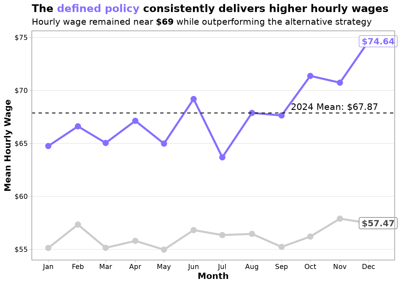
The figure clearly shows that the full policy (orange line) consistently outperforms the baseline (gray line) in every month of 2024. The overall average hourly wage under the policy is $67.87, which is very close to the $69.07 achieved on the 2022–2023 test set (Chapter 10). This confirms that the policy generalises well to a new year.
The monthly averages for the policy are remarkably stable, ranging from about $67 to $69, with no sign of degradation over time. The baseline, in contrast, hovers around $54–$58 per hour, highlighting the large and persistent improvement.
Key Takeaways
The combined policy (trip‑acceptance + optimal start time) is robust and generalises to 2024 data without any retraining. The average hourly wage of $67.87 in 2024 closely matches the $69.07 observed in the 2022–2023 simulation, indicating that the policy captures stable patterns in the ride‑hail market.
The policy outperforms the baseline in every single month of 2024, with a consistent margin of approximately $7–$17 per hour. This eliminates concerns that the gains might be seasonal or driven by specific months.
No retraining is necessary – the models fitted on 2022–2023 data remain effective on 2024 data. This implies that the underlying decision rules (choose Uber, start at night, avoid Mondays/Fridays, and follow the trip‑acceptance tree) are fundamental characteristics of the NYC ride‑hail market, at least over this two‑year horizon.
The policy has passed the out‑of‑sample test and can be confidently recommended for real‑world deployment.