Expanding Geospatial Information

As we saw in the initial exploration, take_current_trip varies across zones, but we know that only providing IDs offers limited context for the models to differentiate between zones. Thus, we enrich the data with geospatial features derived from OpenStreetMap (OSM) to provide deeper insights into each zone.

Here are the steps to follow:

Import data:
- Load NYC taxi zone shapefiles (from TLC, EPSG:2263) and training data.
Extract OSM data:
- Fetch OSM data for Queens, Brooklyn, and Manhattan using key tags.
  - amenity
  - shop
  - office
  - tourism
  - public_transport
  - aeroway
  - emergency
  - sport
  - highway
  - landuse
- Reproject OSM data to EPSG:2263 to match taxi zone CRS.
Spatial joins:
- Link OSM features to taxi zones:
  - Points: Include if within zone.
  - Lines: Include if features are fully contained in zones and for partially intersecting lines, clip the feature to the zone boundary and retain only the overlapping portion.
  - Polygons: Include if features are fully contained in zones and for partially intersecting polygons, clip the feature to the zone boundary and retain only the overlapping portion.
Extract new features:

For each zone and tag:
- Number of OSM points per $mi^2$.
- Total length ($mi$) of OSM lines per $mi^2$.
- Total area ($mi^2$) of OSM polygons per $mi^2$.

Validation:
- Integrate new features and training data
- Define the correlation between new predictors and take_current_trip

Setting up the environment

Loading packages

## To manage relative paths
library(here)

## To transform data that fits in RAM
library(data.table)

## Publish data sets, models, and other R objects
library(pins)
library(qs2)

## To work with spatial data
library(sf)

## To create interactive maps
library(tmap)
tmap_mode("view")

## To download OpenStreetMap data
library(osmdata)

## Transforming distance units
library(units)

## To create general plots
library(ggplot2)

## Custom functions
devtools::load_all()

# Defining the pin boards to use
BoardLocal <- board_folder(here("../NycTaxiPins/Board"))

# Loading params
Params <- yaml::read_yaml(here("params.yml"))
Params$BoroughColors <- unlist(Params$BoroughColors)

Computational Performance

The geospatial processing operations in this document are computationally intensive. Although they could benefit from parallelization with packages like future and future.apply, we’ve opted for a sequential approach with caching via qs2 to maximize reproducibility and maintain code simplicity. Intermediate results are saved after each costly operation to avoid unnecessary recalculations during iterative development.

Define features to import

FeaturesToGet <- c(
  "amenity",
  "shop",
  "office",
  "tourism",
  "public_transport",
  "aeroway",
  "emergency",
  "sport",
  "landuse",
  "highway"
)

Import data

Details on how this data was obtained can be found in the Data Collection Process.

ZonesShapes <-
  pin_read(BoardLocal, "ZonesShapes") |>
  subset(borough %in% names(Params$BoroughColors)) |>
  transform(Shape_Area = st_area(geometry))

SampledData <-
  pin_list(BoardLocal) |>
  grep(pattern = "^OneMonthData", value = TRUE) |>
  sort() |>
  head(12L) |>
  lapply(FUN = pin_read, board = BoardLocal) |>
  rbindlist() |>
  subset(
    select = c("trip_id", "PULocationID", "DOLocationID", "take_current_trip")
  )

Extract OSM data

Defining bounding box

Now we can create a bounding box that encompasses the selected boroughs to efficiently query OSM data for the region we really need.

bb_box <-
  lapply(
    X = paste0(names(Params$BoroughColors), ", NY"),
    FUN = osmdata::getbb
  ) |>
  do.call(what = "cbind") |>
  (\(x) cbind(min = apply(x, 1, min), max = apply(x, 1, max)))()

BoardLocal |> pin_write(bb_box, "bb_box", type = "qs2")

This plot shows the selected boroughs and the taxi zones within them, giving us a visual overview of our geographical units of analysis. The blue rectangle represents the bounding box we defined earlier, encompassing Manhattan (red), Queens (blue), and Brooklyn (green). Each of these boroughs is further divided into smaller taxi zones, which are the primary geographical units for our analysis. The different colors assigned to each borough (defined in the Params$BoroughColors vector) help to visually distinguish them. This initial map confirms that we have correctly loaded the taxi zone shapefile and subsetted it to include only the boroughs of interest for our study.

plot_box(bb_box) +
  tm_shape(ZonesShapes) +
  tm_polygons(
    fill = "borough",
    fill.scale = tm_scale_categorical(values = Params$BoroughColors),
    fill_alpha = 0.6
  )

Of course! Here is a revised description focusing on the benefits of your approach, along with commented code.

A Smart Approach to Getting OSM Data

This section outlines a robust and efficient workflow for fetching, cleaning, and storing geospatial data from OpenStreetMap (OSM). By using custom functions and a caching strategy, we streamline the process and significantly speed up development.

The Power of Custom Functions

Instead of a long, repetitive script, the data retrieval and cleaning process is broken down into two specialized functions: import_osm_feature and tidy_osm_data.

import_osm_feature: This function acts as a dedicated data retriever and pre-processor. For any given feature (like amenities or shops), it not only queries the OSM API but also performs crucial initial cleaning. It discards irrelevant entries and automatically corrects common errors in map geometries (sf::st_make_valid), preventing issues in later analysis. 🗺️
tidy_osm_data: This function takes the raw data and reshapes it into a “tidy” format. By pivoting the data, it organizes features into a consistent structure that is much easier to filter, group, and visualize. It also ensures all data shares the same Coordinate Reference System (CRS), which is essential for accurate spatial analysis. ✨

This modular approach makes the code cleaner, easier to debug, and reusable for other projects.

The Benefit of Caching with `pins`

Querying an API and processing geospatial data are computationally expensive and time-consuming tasks. Doing this every time we run the code is inefficient.

To solve this, we use the pins package to cache our final, processed data object (OsmDataComplete).

Think of it like this: the first time the code runs, it does all the heavy lifting—calling the API, cleaning, and tidying. It then saves the final, ready-to-use result with pin_write. On all subsequent runs, the code can instantly load this saved result using pin_read, bypassing the slow steps entirely. ⚡

This simple caching strategy provides two major benefits:

Speed: It dramatically accelerates the development and testing cycle.
Consistency: It ensures that the data remains consistent between runs, making our results reproducible.

# A custom function to query OSM for a specific feature within a bounding box.
import_osm_feature <- function(feature_name, bb_box) {
  # Build and execute the OSM query.
  osm_list =
    opq(bb_box) |>
    add_osm_feature(feature_name) |>
    osmdata_sf()

  # A list of possible geometry types returned by OSM.
  shape_list =
    c(
      "osm_points",
      "osm_lines",
      "osm_polygons",
      "osm_multilines",
      "osm_multipolygons"
    )

  # Loop through each geometry type to clean the data.
  for (shape_i in shape_list) {
    # Skip if this geometry type is empty.
    if (is.null(osm_list[[shape_i]])) {
      next
    }

    # Clean the data:
    # 1. Remove rows where the feature value is NA (e.g., a shop with no shop type).
    # 2. Keep only the 'name' and the specific feature column for simplicity.
    osm_list[[shape_i]] =
      subset(
        osm_list[[shape_i]],
        !is.na(get(feature_name, inherits = FALSE)),
        select = c("name", feature_name)
      )

    # Check for and fix any invalid map geometries, which can cause errors later.
    not_valid_cases = !sf::st_is_valid(osm_list[[shape_i]])
    if (sum(not_valid_cases) > 0) {
      osm_list[[shape_i]] = sf::st_make_valid(osm_list[[shape_i]])
    }
  }

  # Return the cleaned list of spatial objects.
  return(osm_list)
}

# A function to reshape the OSM data into a tidy format for easier analysis.
tidy_osm_data <- function(osm_sf, crs = NULL) {
  # List of geometry types to process.
  shape_list =
    c(
      "osm_points",
      "osm_lines",
      "osm_polygons",
      "osm_multilines",
      "osm_multipolygons"
    )

  # Loop through each geometry type to tidy it.
  for (shape_i in shape_list) {
    osm_sf[[shape_i]] =
      osm_sf[[shape_i]] |>
      # Remove the original OSM ID as it's not needed for this analysis.
      dplyr::select(-osm_id) |>
      # Pivot the data from a wide format to a long (tidy) format.
      # This creates a 'feature' column and a 'value' column.
      tidyr::pivot_longer(
        !c("name", "geometry"),
        names_to = "feature",
        values_drop_na = TRUE
      )

    # If a target Coordinate Reference System (CRS) is provided, transform the data.
    # This ensures all map layers align correctly.
    if (!is.null(crs)) {
      osm_sf[[shape_i]] = st_transform(osm_sf[[shape_i]], crs = crs)
    }
  }

  return(osm_sf)
}

# Increase the timeout for the API request to prevent errors on large queries.
options(
  httr2_timeout = 60 * 60,
  httr2_connect_timeout = 60 * 60
)

# --- Main Workflow ---
# 1. Apply the 'import_osm_feature' function to every item in 'FeaturesToGet'.
# 2. Combine all the results into a single list.
# 3. Tidy the combined data and set its CRS to match our other spatial data.
OsmDataComplete <-
  lapply(X = FeaturesToGet, FUN = import_osm_feature, bb_box = bb_box) |>
  do.call(what = "c") |>
  tidy_osm_data(crs = st_crs(ZonesShapes)$epsg)

# Cache the final, processed data object to a local pin board.
# 'type = "qs2"' uses a fast and efficient file format.
BoardLocal |> pin_write(OsmDataComplete, "OsmDataComplete", type = "qs2")

# Display the final data.
OsmDataComplete

Spatial joins

We perform two main types of spatial joins to associate the OpenStreetMap features with our taxi zones: first, to identify features entirely within each zone, and second, to identify features that intersect or overlap with the zone boundaries.

Joining elements contained by each zone

Using the st_within function, this section identifies OpenStreetMap features—such as points, lines, polygons, multilinestrings, and multipolygons—that are fully contained within each taxi zone’s boundaries. st_within considers multilinestrings and multipolygons to be within a zone only if all their constituent parts are inside.

PointsWithinZones <-
  OsmDataComplete$osm_points |>
  st_join(y = ZonesShapes, join = st_within, left = FALSE)

LinesWithinZones <-
  OsmDataComplete$osm_lines |>
  st_join(y = ZonesShapes, join = st_within, left = FALSE)

MultiLinesWithinZones <-
  OsmDataComplete$osm_multilines |>
  st_join(y = ZonesShapes, join = st_within, left = FALSE)

PolygonWithinZones <-
  OsmDataComplete$osm_polygons |>
  st_join(y = ZonesShapes, join = st_within, left = FALSE)

MultiPolygonWithinZones <-
  st_make_valid(OsmDataComplete$osm_multipolygons) |>
  st_join(y = ZonesShapes, join = st_within, left = FALSE)

To ensure the accuracy of our spatial joins, we first want to visually inspect the features that were identified as being fully contained within a specific taxi zone. We’ll start by examining zone with LocationID 191.

By examining this map, we can visually confirm that the lines and polygons displayed are indeed located entirely within the boundaries of the chosen taxi zone. This helps us to verify the correctness of our st_within spatial join operation before proceeding with further analysis on these fully contained features.

ZoneToCheck <- 191L

ZonesShapesToCheck <- subset(ZonesShapes, LocationID == ZoneToCheck)
LinesWithinZonesToCheck <- subset(LinesWithinZones, LocationID == ZoneToCheck)
PolygonWithinZonesToCheck <- subset(
  PolygonWithinZones,
  LocationID == ZoneToCheck
)

tm_shape(ZonesShapesToCheck) +
  tm_polygons(fill = "grey") +
  tm_shape(LinesWithinZonesToCheck) +
  tm_lines(col = "feature") +
  tm_shape(PolygonWithinZonesToCheck) +
  tm_polygons(fill = "feature")

Now we can save the save the results.

BoardLocal |>
  pin_write(PointsWithinZones, "PointsWithinZones", type = "qs2")
BoardLocal |>
  pin_write(LinesWithinZones, "LinesWithinZones", type = "qs2")
BoardLocal |>
  pin_write(MultiLinesWithinZones, "MultiLinesWithinZones", type = "qs2")
BoardLocal |>
  pin_write(PolygonWithinZones, "PolygonWithinZones", type = "qs2")
BoardLocal |>
  pin_write(MultiPolygonWithinZones, "MultiPolygonWithinZones", type = "qs2")

Joining lines that are partially contained for each zone.

In this section, we identify OSM features that are not entirely within a taxi zone but do intersect or overlap with its boundary. For lines and multilinestrings, we use st_crosses, which identifies features that intersect the interior of a zone but are not completely contained within it. For polygons and multipolygons, we use st_overlaps, which identifies features that have some area in common with a zone but are not identical to or completely contained within it.

LinesInSeveralZones <-
  OsmDataComplete$osm_lines |>
  st_join(y = ZonesShapes, join = st_crosses, left = FALSE)

MultiLinesInSeveralZones <-
  OsmDataComplete$osm_multilines |>
  st_join(y = ZonesShapes, join = st_crosses, left = FALSE)

PolygonInSeveralZones <-
  OsmDataComplete$osm_polygons |>
  st_join(y = ZonesShapes, join = st_overlaps, left = FALSE)

MultiPolygonInSeveralZones <-
  st_make_valid(OsmDataComplete$osm_multipolygons) |>
  st_join(y = ZonesShapes, join = st_overlaps, left = FALSE)

By visualizing these features, we can confirm that our st_crosses and st_overlaps operations correctly identified the lines and polygons that only partially interact with the selected taxi zone. This is a crucial step before we proceed with the cropping process in the subsequent section, ensuring we only apply the cropping to the features that actually extend beyond the zone boundaries.

LinesInSeveralZonesToCheck <- subset(
  LinesInSeveralZones,
  LocationID == ZoneToCheck
)
PolygonInSeveralZonesToCheck <- subset(
  PolygonInSeveralZones,
  LocationID == ZoneToCheck
)

tm_shape(ZonesShapesToCheck) +
  tm_polygons(fill = "grey") +
  tm_shape(LinesInSeveralZonesToCheck) +
  tm_lines(col = "blue") +
  tm_shape(PolygonInSeveralZonesToCheck) +
  tm_polygons(fill = "feature")

Let’s save the data for future use.

BoardLocal |>
  pin_write(LinesInSeveralZones, "LinesInSeveralZones", type = "qs2")
BoardLocal |>
  pin_write(MultiLinesInSeveralZones, "MultiLinesInSeveralZones", type = "qs2")
BoardLocal |>
  pin_write(PolygonInSeveralZones, "PolygonInSeveralZones", type = "qs2")
BoardLocal |>
  pin_write(
    MultiPolygonInSeveralZones,
    "MultiPolygonInSeveralZones",
    type = "qs2"
  )

Cropping features overlapping multiple zones

This section focuses on refining the geospatial data of lines and polygons that were identified as overlapping multiple taxi zones. The goal is to accurately attribute these features to the specific zone they intersect with.

The apply_intersection_by_id function iterates through each unique taxi zone ID. For each zone, it subsets the lines and polygons that overlap with it and then performs a spatial intersection. This operation effectively “crops” the line or polygon to the exact boundaries of the taxi zone.

This step is crucial for accurately calculating metrics like the length of roads or the area of land use within each zone, as it ensures that only the portion of a feature that lies within a specific zone is considered for that zone.

apply_intersection_by_id <- function(features, shapes) {
  intersection_by_id = function(id, features, shapes) {
    features_sub = subset(features, LocationID == id)
    shapes_sub_geo = subset(shapes, LocationID == id) |> st_geometry()

    new_df = st_intersection(features_sub, shapes_sub_geo)

    return(new_df)
  }

  new_df =
    lapply(
      unique(features$LocationID),
      FUN = intersection_by_id,
      features = features,
      shapes = shapes
    ) |>
    do.call(what = "rbind")

  return(new_df)
}

LinesInSeveralZonesCropped <-
  apply_intersection_by_id(LinesInSeveralZones, ZonesShapes)

MultiLinesInSeveralZonesCropped <-
  apply_intersection_by_id(MultiLinesInSeveralZones, ZonesShapes)

PolygonInSeveralZonesCropped <-
  apply_intersection_by_id(PolygonInSeveralZones, ZonesShapes)

MultiPolygonInSeveralZonesCropped <-
  apply_intersection_by_id(MultiPolygonInSeveralZones, ZonesShapes)

The resulting map shows the blue lines and colored polygons neatly contained within the grey boundary of zone 191. This ensures that when we calculate features like road length or land use area for zone 191, we only consider the portions of these features that actually lie within its boundaries, leading to more accurate analysis.

LinesInSeveralZonesCroppedToCheck <-
  subset(LinesInSeveralZonesCropped, LocationID == ZoneToCheck)

PolygonInSeveralZonesCroppedToCheck <-
  subset(PolygonInSeveralZonesCropped, LocationID == ZoneToCheck)


tm_shape(ZonesShapesToCheck) +
  tm_polygons(fill = "grey") +
  tm_shape(LinesInSeveralZonesCroppedToCheck) +
  tm_lines(col = "blue") +
  tm_shape(PolygonInSeveralZonesCroppedToCheck) +
  tm_polygons(fill = "feature")

After performing those operations, we can save the data for future use.

BoardLocal |>
  pin_write(
    LinesInSeveralZonesCropped,
    "LinesInSeveralZonesCropped",
    type = "qs2"
  )
BoardLocal |>
  pin_write(
    MultiLinesInSeveralZonesCropped,
    "MultiLinesInSeveralZonesCropped",
    type = "qs2"
  )
BoardLocal |>
  pin_write(
    PolygonInSeveralZonesCropped,
    "PolygonInSeveralZonesCropped",
    type = "qs2"
  )
BoardLocal |>
  pin_write(
    MultiPolygonInSeveralZonesCropped,
    "MultiPolygonInSeveralZonesCropped",
    type = "qs2"
  )

Joining objects based on geometry types

After making those changes, we can consolidate all the data to use into 3 geometry types:

POINT
MULTILINESTRING
MULTIPOLYGON

AllPointsZones <- as.data.table(PointsWithinZones)

AllLinesZones <-
  list(
    LinesWithinZones,
    MultiLinesInSeveralZones,
    MultiLinesWithinZones,
    MultiLinesInSeveralZonesCropped
  ) |>
  lapply(FUN = \(df) as.data.table(st_cast(df, to = "MULTILINESTRING"))) |>
  rbindlist(use.names = TRUE)

AllPolygonZones <-
  list(
    PolygonWithinZones,
    PolygonInSeveralZonesCropped,
    MultiPolygonWithinZones,
    MultiPolygonInSeveralZonesCropped
  ) |>
  lapply(FUN = \(df) as.data.table(st_cast(df, to = "MULTIPOLYGON"))) |>
  rbindlist(use.names = TRUE)

BoardLocal |>
  pin_write(AllPointsZones, "AllPointsZones", type = "qs2")
BoardLocal |>
  pin_write(AllLinesZones, "AllLinesZones", type = "qs2")
BoardLocal |>
  pin_write(AllPolygonZones, "AllPolygonZones", type = "qs2")

Extract new features

Number of OSM points per $mi^2$

PointDensityFeatures <-
  AllPointsZones[,
    .N,
    .(
      LocationID = OBJECTID,
      Shape_Area = set_units(Shape_Area, mi^2),
      variable = paste0(toupper(feature), "-", value, "_per_mi2")
    )
  ][, n_per_mi2 := N / as.double(Shape_Area)][, dcast(
    .SD,
    LocationID ~ variable,
    value.var = "n_per_mi2",
    fill = 0L
  )]

BoardLocal |>
  pin_write(PointDensityFeatures, "PointDensityFeatures", type = "qs2")

Total length ($mi$) of OSM lines per $mi^2$

LineDensityFeatures <-
  AllLinesZones[,
    .(total_length = sum(st_length(geometry)) |> set_units(value = mi)),
    .(
      LocationID = OBJECTID,
      Shape_Area = set_units(Shape_Area, mi^2),
      variable = paste0(toupper(feature), "-", value, "_per_mi")
    )
  ][,
    distance_per_mi2 := as.double(total_length) / as.double(Shape_Area)
  ][, dcast(
    .SD,
    LocationID ~ variable,
    value.var = "distance_per_mi2",
    fill = 0L
  )]

BoardLocal |>
  pin_write(LineDensityFeatures, "LineDensityFeatures", type = "qs2")

Total area ($mi^2$) of OSM polygons per $mi^2$

PolygonDensityFeatures <-
  AllPolygonZones[,
    .(total_area = sum(st_area(geometry)) |> set_units(value = mi^2)),
    .(
      LocationID = OBJECTID,
      Shape_Area = set_units(Shape_Area, mi^2),
      variable = paste0(toupper(feature), "-", value)
    )
  ][, area_prop := as.double(total_area) / as.double(Shape_Area)][, dcast(
    .SD,
    LocationID ~ variable,
    value.var = "area_prop",
    fill = 0L
  )]

BoardLocal |>
  pin_write(PolygonDensityFeatures, "PolygonDensityFeatures", type = "qs2")

Validation

Now we just need to consolidate and save all features in a single table and join to the training data.

OmsDensityFeatures <-
  list(PointDensityFeatures, LineDensityFeatures, PolygonDensityFeatures) |>
  Reduce(f = \(x, y) x[y, on = "LocationID"])

PuOmsDensityFeatures <-
  setnames(
    copy(OmsDensityFeatures),
    c("PULocationID", paste0("PU_", names(OmsDensityFeatures)[-1L]))
  )

DoOmsDensityFeatures <-
  setnames(
    copy(OmsDensityFeatures),
    c("DOLocationID", paste0("DO_", names(OmsDensityFeatures)[-1L]))
  )

TrainingSampleOmsDensityFeatures <-
  PuOmsDensityFeatures[
    SampledData,
    on = "PULocationID"
  ][, DoOmsDensityFeatures[.SD, on = "DOLocationID"]]

dim(TrainingSampleOmsDensityFeatures) |> scales::comma()

[1] "242,186" "2,322"

Let’s explore the correlated features.

CorMatrix <- cor(TrainingSampleOmsDensityFeatures[, !c("trip_id")])

BoardLocal |>
  pin_write(CorMatrix, "CorMatrix", type = "qs2")

As we can see, the variables don’t show a strong correlation (<11% for the top cases) with the variable to predict, so we will need to go deeper on feature engineering before using these variables for modeling.

TopOsmCorrelations <-
  as.data.table(CorMatrix, keep.rownames = "variable")[
    order(-abs(take_current_trip)),
    list(
      variable,
      abs_cor = abs(take_current_trip),
      greater_than_0 = take_current_trip > 0
    )
  ][2:16][, variable := reorder(variable, abs_cor, sum)]

BoardLocal |>
  pin_write(TopOsmCorrelations, "TopOsmCorrelations", type = "qs2")

Show the code

ggplot(TopOsmCorrelations) +
  geom_col(
    aes(abs_cor, variable, fill = greater_than_0),
    color = "black",
    linewidth = 0.4
  ) +
  scale_fill_manual(
    values = c("TRUE" = Params$ColorHighlight, "FALSE" = Params$ColorGray)
  ) +
  scale_x_continuous(
    breaks = scales::breaks_width(0.01),
    labels = scales::label_percent(accuracy = 1)
  ) +
  labs(y = "", x = "Absolute Correlation", fill = "Positive Correlation") +
  theme_minimal() +
  theme(legend.position = "top")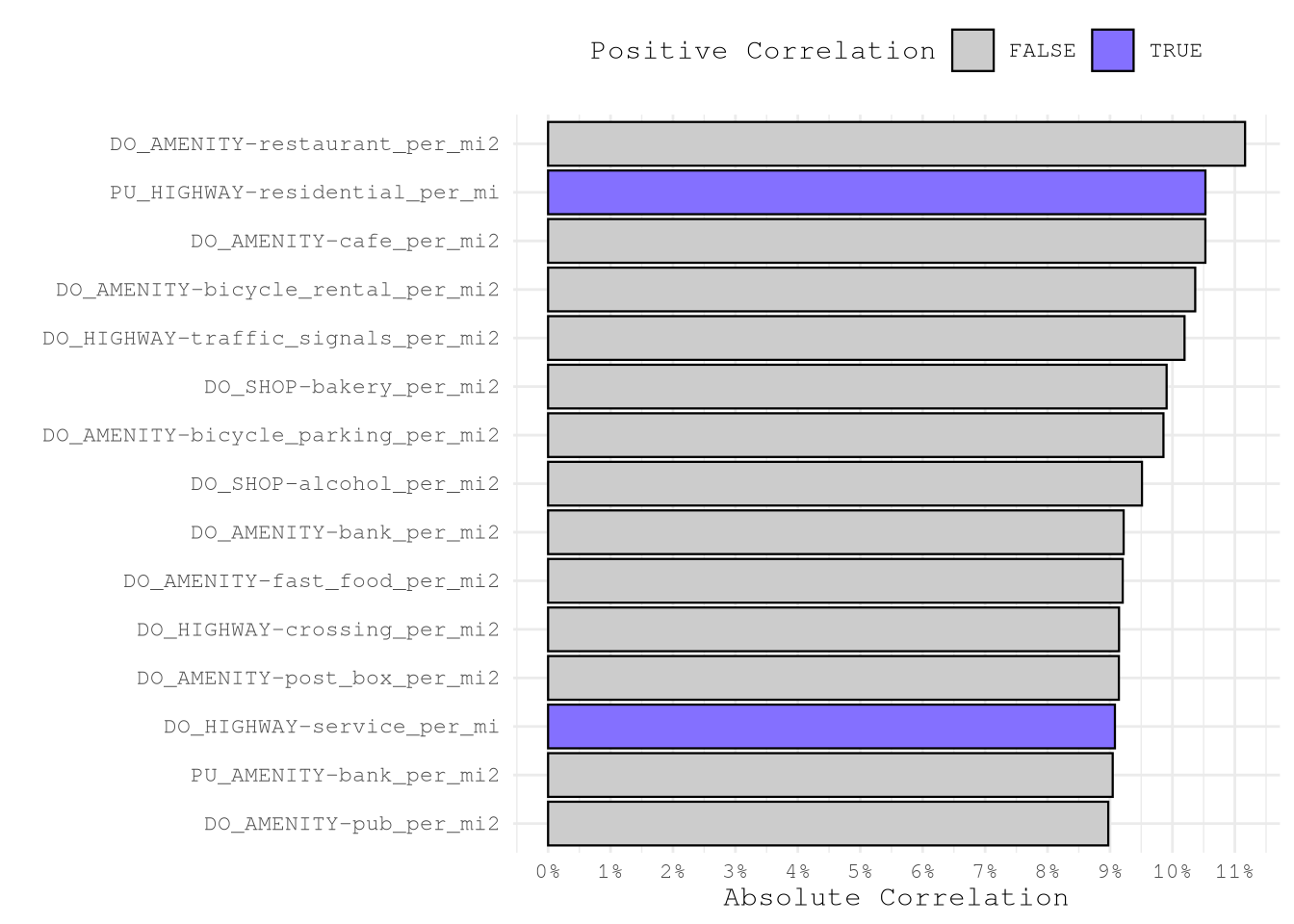

On the other hand, we can also explore in the target variable is correlated with a different median of the new features. As all the variable present different dimensions we are going to scale the variables before calculating the mean and then taking the difference of means.

OsmMedianDiff <-
  TrainingSampleOmsDensityFeatures[,
    lapply(.SD, \(x) {
      if (uniqueN(x) == 1L) x[1L] else median(scale(x, center = FALSE))
    }),
    .SDcols = !c("trip_id", "PULocationID", "DOLocationID"),
    by = "take_current_trip"
  ][, melt(.SD, id.vars = "take_current_trip")][,
    .(not_take_vs_take = diff(value)),
    by = .(variable = as.character(variable))
  ][order(-abs(not_take_vs_take))]

BoardLocal |>
  pin_write(OsmMedianDiff, "OsmMedianDiff", type = "qs2")

In the below chart we can see that for majority of the variables the difference of medians is 0, probably because the feature are near zero variance as doesn’t show very often in many zones, but on the other hand we can see that some features present some $|\text{med}(x)| > 0.1$ that would be important to see in more detail.

Show the code

ggplot(OsmMedianDiff) +
  geom_histogram(aes(not_take_vs_take)) +
  scale_y_continuous(
    transform = scales::new_transform(
      "signed_log10",
      transform = function(x) sign(x) * log10(1 + abs(x)),
      inverse = function(x) sign(x) * (10^(abs(x)) - 1),
      breaks = scales::pretty_breaks()
    ),
    breaks = c(0, 10^(1:4))
  ) +
  labs(y = "count on log10 scale") +
  theme_minimal()

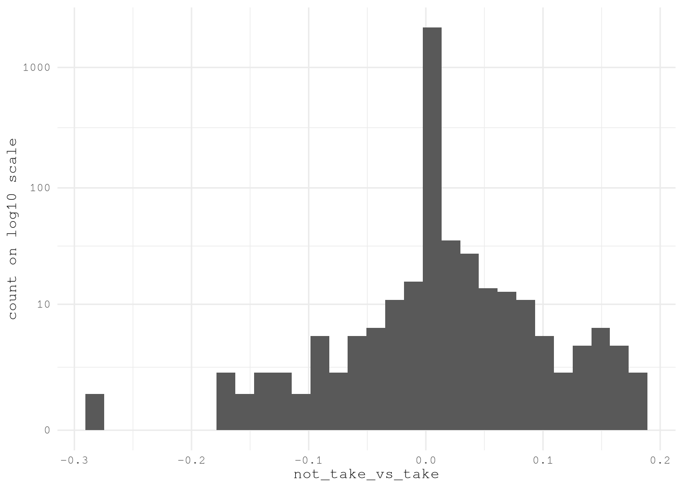
After selecting the to variables to explore, we just need to see

TopOsmMedianDiffFeatures <- OsmMedianDiff[abs(not_take_vs_take) > 0.1, variable]

TopOsmMedianDiff <-
  TrainingSampleOmsDensityFeatures[,
    melt(.SD, id.vars = c("trip_id", "take_current_trip")),
    .SDcols = c("trip_id", "take_current_trip", TopOsmMedianDiffFeatures)
  ][, `:=`(
    variable = factor(variable, levels = rev(TopOsmMedianDiffFeatures)),
    take_current_trip = take_current_trip == 1L
  )][, value := scale(value, center = FALSE), by = "variable"]

BoardLocal |>
  pin_write(TopOsmMedianDiff, "TopOsmMedianDiff", type = "qs2")

Based on the next chart, we can see that the median change based on different factors like:

Variable	Influence of `take_current_trip` (TRUE vs FALSE) on Median
PU_SPORT-american_handball	Median higher when `take_current_trip` is `TRUE`.
DO_AMENITY-bicycle_rental_per_mi2	Median lower when `take_current_trip` is `TRUE`.
PU_AMENITY-school	Median higher when `take_current_trip` is `TRUE`.
DO_AMENITY-bicycle_parking_per_mi2	Median lower when `take_current_trip` is `TRUE`.
PU_AMENITY-restaurant_per_mi2	Median lower when `take_current_trip` is `TRUE`.

Show the code

ggplot(TopOsmMedianDiff) +
  geom_boxplot(aes(x = value, y = variable, fill = take_current_trip)) +
  scale_fill_manual(
    values = c("TRUE" = Params$ColorHighlight, "FALSE" = Params$ColorGray)
  ) +
  scale_x_continuous(
    transform = scales::new_transform(
      "signed_log10",
      transform = function(x) sign(x) * log10(1 + abs(x)),
      inverse = function(x) sign(x) * (10^(abs(x)) - 1),
      breaks = scales::pretty_breaks()
    ),
    labels = scales::label_comma(accuracy = 0.1),
    breaks = c(0, 10^seq(-1, 4, by = 0.25))
  ) +
  labs(x = "", y = "") +
  theme_minimal()

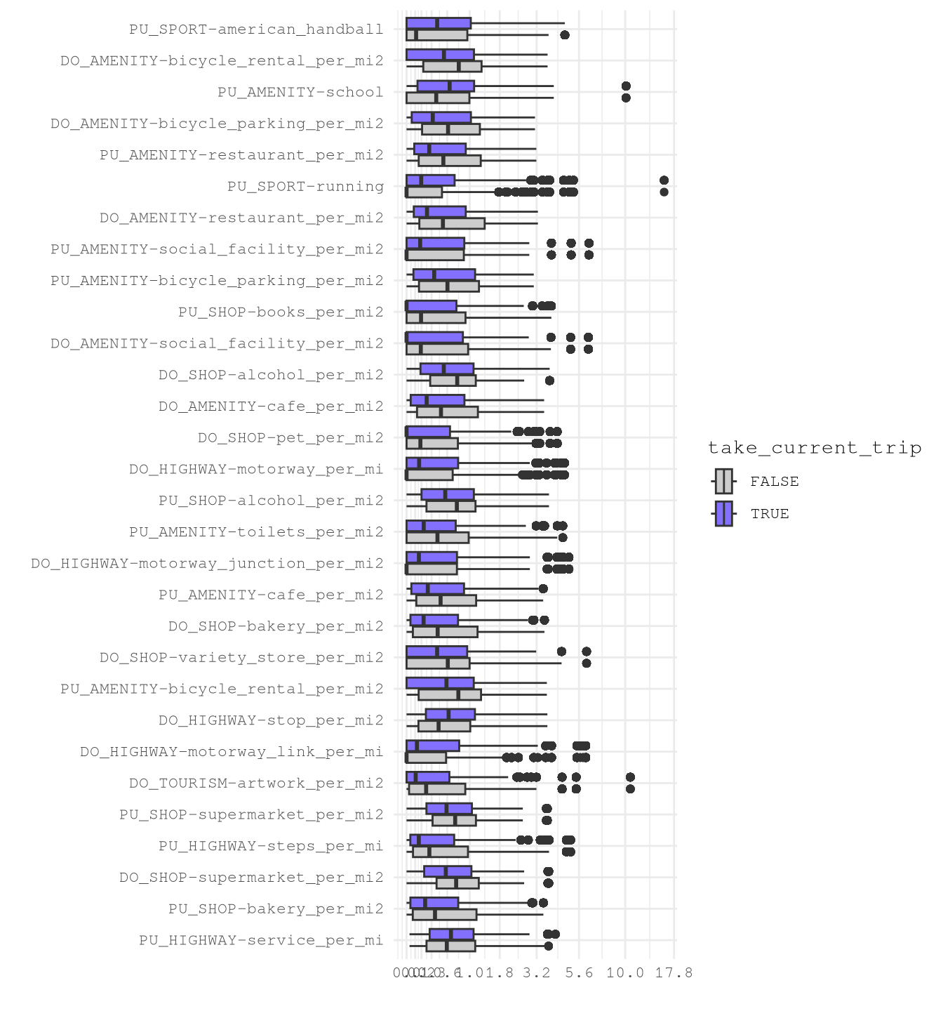
After confirming these promising results we can save the most import features for future use.

OmsDensityFeatures <-
  c("LocationID", sub("(PU|DO)_", "", TopOsmMedianDiffFeatures)) |>
  unique()

BoardLocal |> pin_write(OmsDensityFeatures, "OmsDensityFeatures", type = "qs2")

Conclusion

We know that these features will be useful for modeling, especially for finding correlations with weekdays and hours.

It’s important to take in consideration that the data is right skewed and present some high-leverage points that will need to be solved depending on the model to select.

Setting up the environment

Loading packages

Define features to import

Import data

Extract OSM data

Defining bounding box

A Smart Approach to Getting OSM Data

The Power of Custom Functions

The Benefit of Caching with pins

Spatial joins

Joining elements contained by each zone

Joining lines that are partially contained for each zone.

Cropping features overlapping multiple zones

Joining objects based on geometry types

Extract new features

Validation

Conclusion

The Benefit of Caching with `pins`