Simulation-Based Estimation of the Baseline Hourly Wage for NYC Taxi Drivers

Defining the baseline from the available data is challenging because the data lack a unique identifier for direct estimation. However, we can run a simulation to estimate the baseline value together with a confidence interval.

Simulation Assumptions

The simulation is built on the following assumptions regarding taxi drivers:

They can start working:
- From any zone in Manhattan, Brooklyn, or Queens (the most active boroughs).
- In any month, on any weekday, and at any hour.
The TLC license number (taxi company) must remain constant for all trips within a workday.
Only wheelchair‑accessible vehicles can accept trips that request a wheelchair‑accessible vehicle.
Because we cannot determine whether each zone has more active taxis than passengers, we assume that there are always more passengers than taxis. Consequently, each taxi driver picks a random qualifying trip from the candidates found within the current search radius and time window (respecting WAV compatibility, same taxi company, and the daily time limit).
Taxis search for trips based on waiting time and accept the first trip found within an expanding radius:
- 0–1 minute: search within a 1‑mile radius.
- 1–3 minutes: if no trip is found, expand search to a 3‑mile radius.
- 3–5 minutes: if still no trip, expand to a 5‑mile radius.
- Continue adding 2 miles every two minutes until a trip is found.
Drivers take a 30‑minute break after 4 hours of work, but only after completing the current trip.
They will accept their last trip after working 8 hours (the 30‑minute break is not counted toward the 8 hours).

Formalizing the Simulation

Based on the rules above, we define a mathematical model following the framework described by Warren B. Powell (2022) in Sequential Decision Analytics and Modeling: Modeling with Python.

Mathematical Model Definition

Based on the simulation assumptions (taxi drivers can start in any active borough/zone/month/weekday/hour, TLC license is fixed per workday, WAV rules apply, more passengers than taxis so the driver picks a random qualifying trip from the candidates that satisfy the radius/time/WAV/company/day-limit constraints, search radius expands with waiting time: 1 mile for 0–1 min, 3 miles for 1–3 min, 5 miles for 3–5 min, then +2 miles every two minutes, 30-minute break after exactly 4 hours of work but only after finishing the current trip, last trip accepted even if it finishes after the 8-hour limit), we formalize the problem using the sequential decision framework.

State variables $S_t^n$ for the $n$-th sample

The reservoir-sampled trip $I_0^n$ is used only to seed the simulation. It is not counted in earnings or working hours. Its attributes determine:

Vehicle Profile
- Taxi Company ($\text{Taxi\_Company}^n$): hvfhs_license_num of $I_0^n$
- Taxi is WAV ($\text{Taxi\_Is\_WAV}^n$): wav_match_flag of $I_0^n$
Shift Constraints
- Limit To Take Trips ($\text{Limit\_To\_Take\_Trips}^n$): end time of $I_0^n$ + 8 hours + 30 minutes
- Time To Take Break ($\text{Time\_To\_Take\_Break}^n$): end time of $I_0^n$ + 4 hours
Initial Operational State
- Taken Break ($\text{Taken\_Break}_0^n$) = FALSE
- Current Time ($\text{Current\_Time}_0^n$) = end time of $I_0^n$ (driver is free and ready to search)
- Current Position Zone ($\text{Current\_Zone}_0^n$) = DOLocationID of $I_0^n$
Initial Search Policy
- Trip Time Limit ($\text{Trip\_Time\_Limit}_0^n$) = $\text{Current\_Time}_0^n$ + 1 minute
- Trip Distance Limit ($\text{Trip\_Dist\_Limit}_0^n$) = 1 mile
\[ S_0^n = \begin{pmatrix} \left. \begin{array}{l} \text{Taxi\_Company}^n \\ \text{Taxi\_Is\_WAV}^n \end{array} \right\} \text{Vehicle Profile} \\ \left. \begin{array}{l} \text{Limit\_To\_Take\_Trips}^n \\ \text{Time\_To\_Take\_Break}^n \end{array} \right\} \text{Shift Constraints} \\ \left. \begin{array}{l} \text{Taken\_Break}_0^n \\ \text{Current\_Time}_0^n \\ \text{Current\_Zone}_0^n \end{array} \right\} \text{Initial Operational State} \\ \left. \begin{array}{l} \text{Trip\_Time\_Limit}_0^n \\ \text{Trip\_Dist\_Limit}_0^n \end{array} \right\} \text{Initial Search Policy} \end{pmatrix} \]
- Dynamic state variables $S_t^n$
  - Current Time ($\text{Current\_Time}_t^n$): The date and time when the driver is searching for a new trip.
  - Current Position Zone ($\text{Current\_Zone}_t^n$): The zone code where the driver is currently located.
  - Taken Break ($\text{Taken\_Break}_t^n$): FALSE until the break is taken, then TRUE.
  - Trip Time Limit ($\text{Trip\_Time\_Limit}_t^n$): The time until which the driver searches for a trip within the current distance limit. Updated by adding 1 or 2 minutes to $\text{Current\_Time}_t^n$ depending on previous search outcomes.
  - Trip Distance Limit ($\text{Trip\_Dist\_Limit}_t^n$): The radius (in miles) within which the driver searches for the next trip. Increases as $\text{Trip\_Time\_Limit}_t^n$ moves further from $\text{Current\_Time}_t^n$.
\[ S_t^n = \begin{pmatrix} \left. \begin{array}{l} \text{Current\_Time}_t^n \\ \text{Current\_Zone}_t^n \\ \text{Taken\_Break}_t^n \end{array} \right\} \text{\small Operational Tracking} \\ \left. \begin{array}{l} \text{Trip\_Time\_Limit}_t^n \\ \text{Trip\_Dist\_Limit}_t^n \end{array} \right\} \text{\small Search Policy State} \end{pmatrix} \]

Decision variables $x_t$
The driver decides whether to accept a sampled trip based on current location and time. Hence $x_t$ is a binary variable defined by the policy: \[ x_t = X^\pi(S_t^n \mid \theta) \]

Where $\pi = (f, \theta)$ is the policy; for the baseline, the driver picks a trip uniformly at random from all qualifying trips that satisfy the radius/time/WAV/company/day-limit constraints.
Exogenous information $W_{t+1}^n$
After completing a trip, the following variables are observed from the data:
- Trip End Time ($\text{Trip\_End\_Time}_{t+1}^n$): The date and time when the trip ends: request_datetime + trip_time of the accepted trip.
- Trip End Zone ($\text{Trip\_End\_Zone}_{t+1}^n$): The zone where the trip ends, taken from the DOLocationID of the accepted trip.
- Trip Earning ($\text{Trip\_Earning}_{t+1}^n$): The total earnings from the trip: driver_pay + tips of the accepted trip.
\[ W_{t+1}^n = \big( \text{Trip\_End\_Time}_{t+1}^n,\; \text{Trip\_End\_Zone}_{t+1}^n,\; \text{Trip\_Earning}_{t+1}^n \big) \]
Transition function $S^M(S_t^n, x_t, W_{t+1}^n)$
After a trip is taken ($x_t = 1$), the state variables are updated as follows (if $x_t = 0$, the search limits are expanded according to the rules and the driver continues searching without changing position or taking a break):

\[ \text{Current\_Time}_{t+1}^n = \text{Trip\_End\_Time}_{t+1}^n \] \[ \text{Current\_Zone}_{t+1}^n = \text{Trip\_End\_Zone}_{t+1}^n \]

If the trip just completed causes the break time to be exceeded and the break has not yet been taken: \[ \begin{aligned} &\textbf{if } \big( \text{Current\_Time}_{t+1}^n > \text{Time\_To\_Take\_Break}^n \text{ and } \neg \text{Taken\_Break}_t^n \big) \textbf{ then} \\ &\quad \text{Current\_Time}_{t+1}^n \leftarrow \text{Current\_Time}_{t+1}^n + 30 \text{ min} \\ &\quad \text{Taken\_Break}_{t+1}^n \leftarrow \text{TRUE} \\ &\textbf{else} \\ &\quad \text{Taken\_Break}_{t+1}^n \leftarrow \text{Taken\_Break}_t^n \\ &\textbf{end if} \end{aligned} \]

Reset the search window: \[ \text{Trip\_Time\_Limit}_{t+1}^n = \text{Current\_Time}_{t+1}^n + 1\;\text{min} \] \[ \text{Trip\_Dist\_Limit}_{t+1}^n = 1\;\text{mile} \]
Objective function

The daily hourly wage is computed for the full workday starting from the moment the driver is free after the seeding trip (even though the seeding trip itself contributes neither earnings nor hours to the sum):

\[ F^{\pi^\tau}(S_0^n) = \mathbb{E}\left[ \frac{\sum_{t=1}^{T^n} (\text{Trip\_Earning}_{t+1}^n \cdot x_t)} {(\text{RequestTime}_{T^n}^n + \text{trip\_time}_{T^n}^n) - \text{EndTime}_{I_0^n}} \;\middle|\; S_0^n \right] \]

Where $\text{EndTime}_{I_0^n}$ is the drop-off time of the reservoir-sampled seeding trip $I_0^n$, $T^n$ is the number of policy-accepted trips, and earnings are summed only over the policy-driven trips (seeding trip excluded).

Last-trip overrun rule
Any candidate trip whose request_datetime $\leq$ $\text{Limit\_To\_Take\_Trips}^n$ (or whose request falls inside the current search window) is eligible, even if its drop-off time exceeds $\text{Limit\_To\_Take\_Trips}^n$. The driver accepts this final trip and the shift ends at the actual drop-off time. This implements assumption 7 exactly.

Uncertainty Model

Uncertainty enters the model both through the initial state $S_0^n$ and through the exogenous information process $W_1^n, \dots, W_{T^n}^n$.

Let $\mathcal{D}$ be the full historical dataset of trips (each trip identified by its unique index $i$).

Through the initial state $S_0^n$:
Sample the starting trip index $I_0^n$ uniformly at random from all feasible starting trips in $\mathcal{D}$. All components of $S_0^n$ are computed directly from the attributes of trip $I_0^n$.
Through the exogenous information process $W_{t+1}^n$:
Given the current state $S_t^n$, define the set of candidate trips that satisfy the simulation rules (time window, radius, WAV compatibility, same Taxi_Company, etc.):

\[ \begin{aligned} \mathcal{C}_t^n = \Big\{ i \in \mathcal{D} \mid \text{ } & \text{request\_datetime}_i \geq \text{Current\_Time}_t^n, \\ & \text{request\_datetime}_i \leq \text{Trip\_Time\_Limit}_t^n, \\ & \text{dist}(\text{PULocationID}_i, \text{Current\_Zone}_t^n) \leq \text{Trip\_Dist\_Limit}_t^n, \\ & \text{req\_datetime}_i \leq \text{Limit\_To\_Take\_Trips}^n, \\ & \text{and all other constraints hold} \Big\} \end{aligned} \]

If $|\mathcal{C}_t^n| \geq 1$, select the trip index purely randomly:

\[ I_{t+1}^n \sim \text{Uniform}(\mathcal{C}_t^n) \]

Then extract the exogenous information directly from the selected trip:

\[ W_{t+1}^n = \Big( \text{request\_datetime}_{I_{t+1}^n} + \text{trip\_time}_{I_{t+1}^n}, \;\; \text{DOLocationID}_{I_{t+1}^n}, \;\; \text{driver\_pay}_{I_{t+1}^n} + \text{tips}_{I_{t+1}^n} \Big) \]

If $\mathcal{C}_t^n = \emptyset$, expand the search limits (add 1–2 minutes and 2 miles) and repeat until a candidate appears — the waiting time remains purely data-driven.

The candidate set $\mathcal{C}_t^n$ is built exactly as in the original definition.

Because of the while guard and the last-trip rule above, the simulation naturally allows the final trip to overrun the nominal 8-hour limit.

Evaluating policies

We will use 5 seeds to get the average result of each $S_0^n$ in $N$. For each initial state sample $S_0^n$ ($n = 1, \dots, N$), the simulation is run 5 times with 5 different random seeds (different realizations of the index selections).

The objective value for that $S_0^n$ is the average over the 5 seeds. The overall baseline estimate (with confidence interval) is then the average (and standard error) across all $N$ initial samples. This Monte-Carlo procedure with fixed seeds provides a reproducible estimate of the expectation in the objective function.

sample.int(1e4, 5)
#> [1] 8199   50 7450 1430 9370

Running trips simulation

The function simulate_trips() (loaded via devtools::load_all()) is the exact computational realization of the sequential-decision process described above.

For every initial state $S_0^n$ (one per reservoir-sampled trip):
- It uses $I_0^n$ only to fix the vehicle profile, starting zone, free time, and shift limits.
- It never includes the earnings or hours of $I_0^n$.
- The while loop searches for and accepts only policy-driven trips ($t \geq 1$).
- The returned table therefore contains precisely the trajectory needed for the updated objective function.

Loading the functions to use.

library(here)
library(scales)
library(ggplot2)
library(data.table)
library(lubridate)
library(infer)
library(DBI)
library(duckdb)
library(glue)
library(pins)
library(qs2)
library(sf)
library(units)

## Custom functions
devtools::load_all()

## Defining the print params to use in the report
options(datatable.print.nrows = 15, digits = 4)

# Defining the pin boards to use
BoardLocal <- board_folder(here("../NycTaxiPins/Board"))

# Loading params
Params <- yaml::read_yaml(here("params.yml"))

Importing zones shapes

ZonesShapes <-
  pin_read(BoardLocal, "ZonesShapes") |>
  subset(borough %in% names(Params$BoroughColors))

Defining the mean distance in miles for all zone combinations.

ZoneDistMatrix <-
  st_centroid(ZonesShapes) |>
  st_distance() |>
  units::set_units(mi) |>
  units::drop_units()

colnames(ZoneDistMatrix) <- ZonesShapes$LocationID
rownames(ZoneDistMatrix) <- ZonesShapes$LocationID

PointMeanDistance <-
  ZoneDistMatrix |>
  as.data.table(keep.rownames = "PULocationID") |>
  melt(
    id.vars = "PULocationID",
    variable.name = "DOLocationID",
    value.name = "trip_miles_mean",
    variable.factor = FALSE
  )

PointMeanDistance[, `:=`(
  PULocationID = sub("^X", "", PULocationID) |> as.double(),
  DOLocationID = as.double(DOLocationID)
)]

pin_write(BoardLocal, PointMeanDistance, "PointMeanDistance", type = "qs2")

Saving the results in the db.

con <- dbConnect(duckdb(), dbdir = here("../NycTaxiBigFiles/my-db.duckdb"))
dbWriteTable(con, "PointMeanDistance", PointMeanDistance, overwrite = TRUE)
dbDisconnect(con, shutdown = TRUE)

Selecting at random the trip to start each simulation.

# Sampling 1,061 trips from db
SimulationStartDayQuery <- "
SELECT t1.*
FROM NycTrips t1
INNER JOIN PointMeanDistance t2
  ON t1.PULocationID = t2.PULocationID AND
     t1.DOLocationID = t2.DOLocationID
WHERE t1.year = 2023
      AND t1.trip_time >= (60 * 2)
      AND t1.trip_miles > 0
      AND t1.driver_pay > 0
USING SAMPLE reservoir(1061 ROWS) REPEATABLE (1144);
"
con <- dbConnect(duckdb(), dbdir = here("../NycTaxiBigFiles/my-db.duckdb"))
SimulationStartDay <- dbGetQuery(con, SimulationStartDayQuery)
dbDisconnect(con, shutdown = TRUE)

# Saving results
setDT(SimulationStartDay)
pin_write(BoardLocal, SimulationStartDay, "SimulationStartDay", type = "qs2")

pillar::glimpse(SimulationStartDay)

Rows: 1,061
Columns: 28
$ trip_id              <dbl> 232477404, 410212402, 371998117, 342529321, 30591…
$ hvfhs_license_num    <chr> "HV0005", "HV0003", "HV0003", "HV0003", "HV0003",…
$ dispatching_base_num <chr> "B03406", "B03404", "B03404", "B03404", "B03404",…
$ originating_base_num <chr> NA, "B03404", "B03404", "B03404", "B03404", "B034…
$ request_datetime     <dttm> 2023-02-03 15:19:29, 2023-11-08 23:16:18, 2023-0…
$ on_scene_datetime    <dttm> NA, 2023-11-08 23:19:04, 2023-09-11 09:19:06, 20…
$ pickup_datetime      <dttm> 2023-02-03 15:22:47, 2023-11-08 23:19:55, 2023-0…
$ dropoff_datetime     <dttm> 2023-02-03 15:39:01, 2023-11-09 00:00:33, 2023-0…
$ PULocationID         <dbl> 227, 166, 138, 161, 36, 203, 102, 143, 90, 219, 1…
$ DOLocationID         <dbl> 181, 225, 97, 261, 37, 205, 36, 50, 162, 132, 89,…
$ trip_miles           <dbl> 2.140, 13.210, 8.710, 6.490, 1.460, 4.160, 1.286,…
$ trip_time            <dbl> 974, 2438, 2736, 1521, 572, 1015, 519, 253, 1150,…
$ base_passenger_fare  <dbl> 19.35, 44.07, 39.94, 36.94, 10.42, 14.97, 10.10, …
$ tolls                <dbl> 0.00, 6.94, 0.00, 0.00, 0.00, 0.00, 0.00, 0.00, 0…
$ bcf                  <dbl> 0.58, 1.40, 1.17, 1.02, 0.31, 0.45, 0.28, 0.23, 0…
$ sales_tax            <dbl> 1.72, 4.53, 3.77, 3.28, 0.92, 1.33, 0.90, 0.73, 1…
$ congestion_surcharge <dbl> 0.00, 0.00, 0.00, 2.75, 0.00, 0.00, 0.00, 2.75, 2…
$ airport_fee          <dbl> 0.0, 0.0, 2.5, 0.0, 0.0, 0.0, 0.0, 0.0, 0.0, 2.5,…
$ tips                 <dbl> 3.90, 5.69, 0.00, 4.39, 0.00, 0.00, 0.00, 1.00, 0…
$ driver_pay           <dbl> 11.78, 40.75, 37.16, 22.83, 7.79, 18.12, 6.62, 5.…
$ shared_request_flag  <chr> "N", "N", "N", "N", "N", "N", "N", "N", "N", "N",…
$ shared_match_flag    <chr> "N", "N", "N", "N", "N", "N", "N", "N", "N", "N",…
$ access_a_ride_flag   <chr> "N", "N", " ", " ", " ", " ", "N", "N", " ", " ",…
$ wav_request_flag     <chr> "N", "N", "N", "N", "N", "N", "N", "N", "N", "N",…
$ wav_match_flag       <chr> "N", "N", "N", "N", "N", "Y", "N", "N", "N", "N",…
$ month                <chr> "02", "11", "09", "07", "05", "03", "11", "12", "…
$ year                 <dbl> 2023, 2023, 2023, 2023, 2023, 2023, 2023, 2023, 2…
$ performance_per_hour <dbl> 57.95, 68.57, 48.89, 64.43, 49.03, 64.27, 45.92, …

We can also confirm that the sample satisfy the initial restrictions:

All trips are from 2023.

SimulationStartDay[, .N, year]

    year     N
   <num> <int>
1:  2023  1061

The trips begin and end on the expected boroughs.

setDT(ZonesShapes)

merge(
  ZonesShapes[
    SimulationStartDay,
    on = c("LocationID" = "PULocationID"),
    .(n_start_trips = .N),
    by = .(Borough = borough)
  ],
  ZonesShapes[
    SimulationStartDay,
    on = c("LocationID" = "DOLocationID"),
    .(n_end_trips = .N),
    by = .(Borough = borough)
  ],
  by = "Borough",
  all = TRUE
)

Key: <Borough>
     Borough n_start_trips n_end_trips
      <char>         <int>       <int>
1:  Brooklyn           340         334
2: Manhattan           482         481
3:    Queens           244         251

Running the simulation.

con <- dbConnect(duckdb(), dbdir = here("../NycTaxiBigFiles/my-db.duckdb"))

SimulationHourlyWage <- simulate_trips(
  con,
  SimulationStartDay,
  seeds = c(8199, 50, 7450, 1430, 9370)
)

dbDisconnect(con, shutdown = TRUE)

pin_write(
  BoardLocal,
  SimulationHourlyWage,
  "SimulationHourlyWage",
  type = "qs2"
)

Confirming simulation results

Now we just need to take the mean and standard desviation of each trip see the results of the simulation for each initial condition.

SimulationHourlyWage[
  SimulationStartDay,
  on = c("simulation_id" = "trip_id"),
  initial_day_time := request_datetime + lubridate::seconds(trip_time)
]

SimulationHourlyWageSummary <-
  SimulationHourlyWage[,
    .(
      n_trips = .N,
      total_hours_worked = difftime(
        max(sim_dropoff_datetime),
        min(initial_day_time),
        unit = "hours"
      ) |>
        as.double(),
      total_earnings = sum(sim_driver_pay, na.rm = TRUE) +
        sum(sim_tips, na.rm = TRUE)
    ),
    by = c("simulation_id", "simulation_seed")
  ][, daily_hourly_wage := total_earnings / total_hours_worked][,
    j = c(
      setNames(lapply(.SD, mean), paste0(names(.SD), "_mean")),
      setNames(lapply(.SD, sd), paste0(names(.SD), "_sd"))
    ),
    .SDcols = !c("simulation_seed"),
    by = "simulation_id"
  ]


setcolorder(
  SimulationHourlyWageSummary,
  c(
    "simulation_id",
    paste0("n_trips", c("_mean", "_sd")),
    paste0("total_hours_worked", c("_mean", "_sd")),
    paste0("total_earnings", c("_mean", "_sd")),
    paste0("daily_hourly_wage", c("_mean", "_sd"))
  )
)

head(SimulationHourlyWageSummary)

   simulation_id n_trips_mean n_trips_sd total_hours_worked_mean
           <num>        <num>      <num>                   <num>
1:     232477404         30.2     4.3243                   8.598
2:     410212402         26.0     0.7071                   8.776
3:     371998117         21.0     2.3452                   8.744
4:     342529321         23.6     1.1402                   8.555
5:     305917160         29.0     2.6458                   8.801
6:     264601024         29.8     3.9623                   8.683
   total_hours_worked_sd total_earnings_mean total_earnings_sd
                   <num>               <num>             <num>
1:               0.14524               397.8             62.31
2:               0.26401               520.1             80.47
3:               0.15620               434.6             38.29
4:               0.06854               477.2             29.09
5:               0.16554               561.2             18.49
6:               0.19292               491.7             32.47
   daily_hourly_wage_mean daily_hourly_wage_sd
                    <num>                <num>
1:                  46.25                7.193
2:                  59.39               10.233
3:                  49.70                4.267
4:                  55.79                3.564
5:                  63.78                2.262
6:                  56.63                3.472

Here we can confirm that was the simulations ended after 8.5 hours.

Show the code

ggplot(SimulationHourlyWageSummary) +
  geom_histogram(aes(total_hours_worked_mean), bins = 30) +
  scale_x_continuous(n.breaks = 10) +
  labs(title = "Distribution of mean of hours worked", x = "Hours Worked") +
  theme_minimal(base_family = Params$BaseFontFamily) +
  theme(plot.title = element_text(face = "bold", size = 15))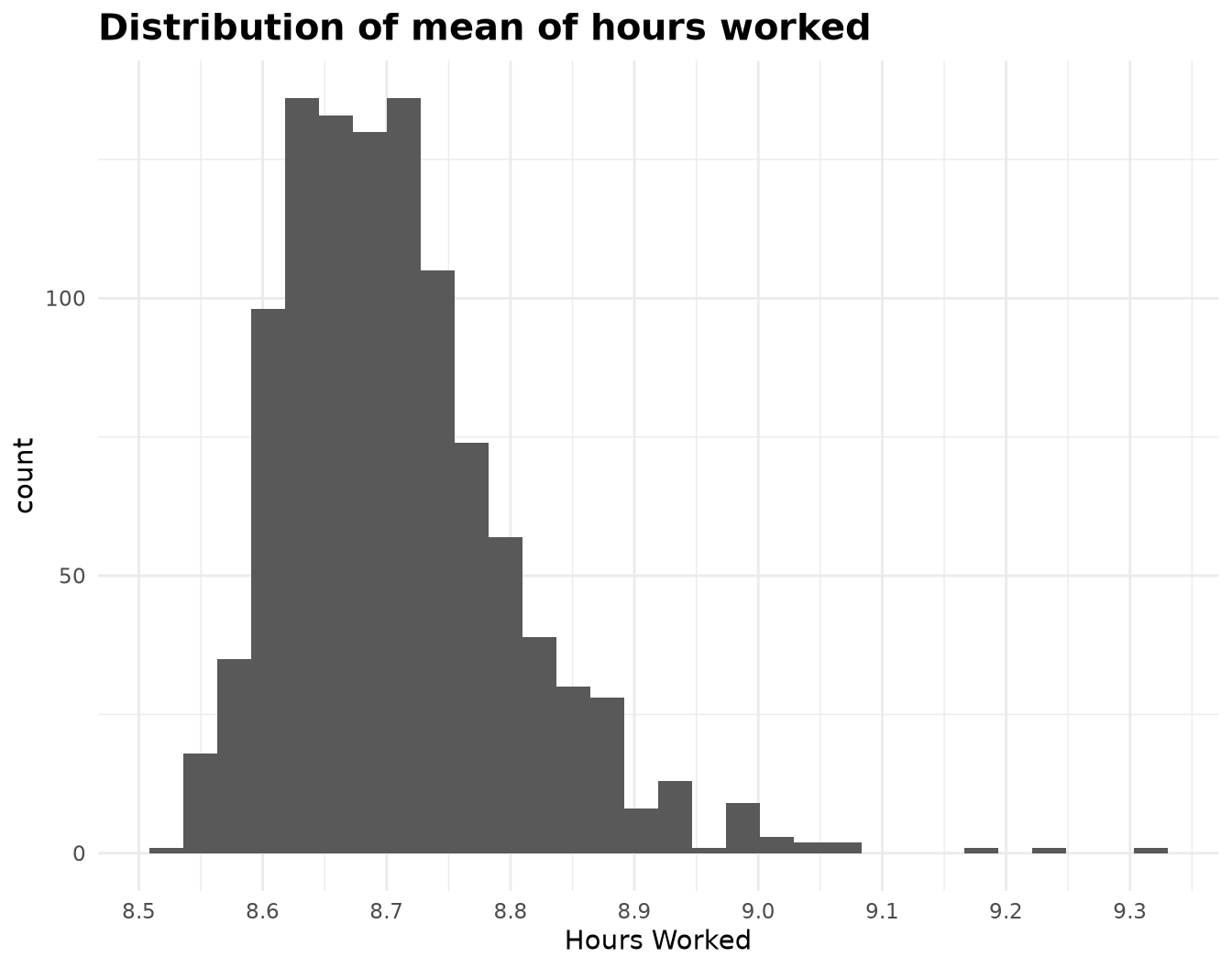

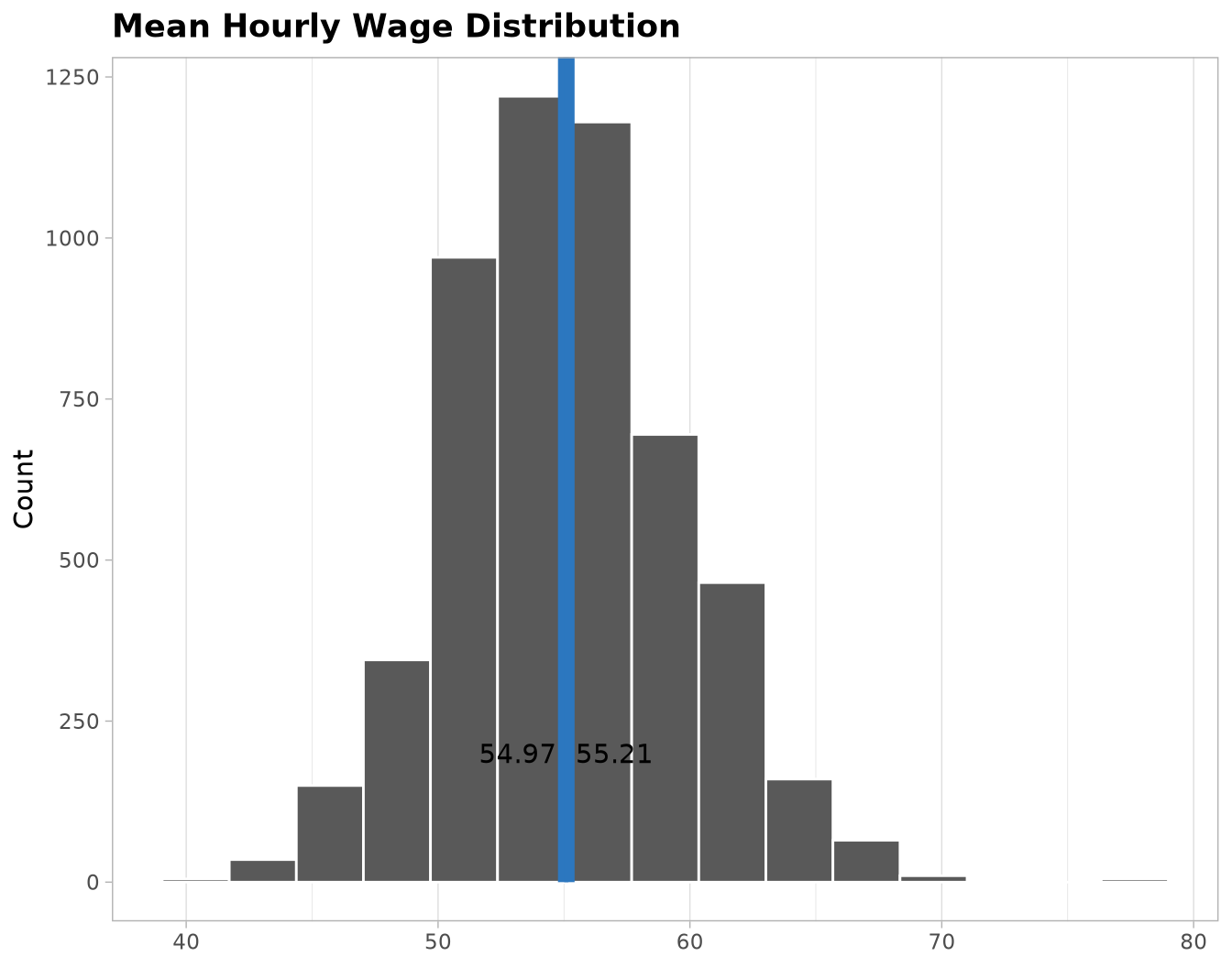
Defining a Confidence Interval

After simulating 1,061 independent starting conditions (each averaged over 5 reproducible seeds), we can use the Monte Carlo results to infer the distribution of the mean Daily Hourly Wage for any day.

Show the code

overall_mean <- mean(SimulationHourlyWageSummary$daily_hourly_wage_mean)
se_mean <- sd(SimulationHourlyWageSummary$daily_hourly_wage_mean) /
  sqrt(nrow(SimulationHourlyWageSummary))
ci_lower <- overall_mean - qnorm(0.975) * se_mean
ci_upper <- overall_mean + qnorm(0.975) * se_mean

SimulationInterval <- data.table(lower_ci = ci_lower, upper_ci = ci_upper)

SimulationVisData <- SimulationHourlyWageSummary[, .(
  replicate = simulation_id,
  stat = daily_hourly_wage_mean
)] |>
  as.data.frame()

attr(SimulationVisData, "class") <- c("infer", "data.frame")
attr(SimulationVisData, "type") <- "bootstrap" # satisfies the switch()

visualize(SimulationVisData) +
  shade_ci(
    endpoints = c(
      lower_ci = SimulationInterval$lower_ci,
      upper_ci = SimulationInterval$upper_ci
    ),
    color = "#2c77BF",
    fill = "#2c77BF"
  ) +
  annotate(
    geom = "text",
    y = 200,
    x = c(
      SimulationInterval[1L][[1L]] - 1.8,
      SimulationInterval[1L][[2L]] + 1.8
    ),
    label = unlist(SimulationInterval) |> comma(accuracy = 0.01)
  ) +
  labs(title = "Mean Hourly Wage Distribution", y = "Count") +
  theme_light(base_family = Params$BaseFontFamily) +
  theme(
    panel.grid.minor.y = element_blank(),
    panel.grid.major.y = element_blank(),
    plot.title = element_text(face = "bold"),
    axis.title.x = element_blank()
  )

Business Case

! The hash of pin "BaseLineHourlyWage" has not changed.
• Your pin will not be stored.

Based on the simulation’s results we can confirm that the average earnings for a taxi driver per hour goes between $54.82 and $55.37 with 95% confidence with a mean of $55.09 dollars per hour.

That means that for incrementing 20% the new rate must be at least $66.11 dollars per hour, which translate to be an increase of $1,762.92 every month.