## To manage relative paths
library(here)
library(pins)
library(qs2)

## Manipulate data
library(data.table)
library(DBI)
library(duckdb)
library(lubridate)
library(timeDate)

## To run predictions
library(tidymodels)

## To show results
library(ggtext)
library(scales)

## Custom functions & board
devtools::load_all()
BoardLocal <- board_folder(here("../NycTaxiPins/Board"))

# Loading params
Params <- yaml::read_yaml(here("params.yml"))

# Sampled data (Chapter 4)
SimulationStartDay <- pin_read(
  BoardLocal,
  name = "SimulationStartDay"
)
SimulationHourlyWage <- pin_read(
  BoardLocal,
  name = "SimulationHourlyWage"
)

BaseLineHourlyWage <- pin_read(BoardLocal, "BaseLineHourlyWage")

# Production workflow (Chapter 8)
XgboostFinalWorkflowTailorFitted <- pin_read(
  BoardLocal,
  name = "XgboostFinalWorkflowTailorFitted"
)

InitalBestThresholdValue <- pin_read(BoardLocal, "BestThresholdValue")From Predictions to Policies: Integrating ML into Stochastic Optimization
Evaluating the ADP Policy in Full-Day Monte-Carlo Simulation
This chapter closes the Approximate Dynamic Programming (ADP) loop. We convert the probabilistic XGBoost classifier into a tunable threshold policy \(\pi^\tau\) and re-evaluate it inside the exact same full-day empirical Monte-Carlo simulator used for the baseline in Chapter 4. The result is a directly comparable hourly-wage lift under the identical data-driven uncertainty model \(\mathcal{C}_t^n\).
Updated Mathematical Model
The state, exogenous information, and transition functions remain identical to Chapter 4. Only the decision rule changes.
Decision variable
\[
x_t = \mathbb{I} \{ \hat{p}_t(S_t) \ge \tau \}
\]
where \(\hat{p}_t(S_t)\) is the XGBoost probability that the current offered trip (sampled from \(\mathcal{C}_t^n\)) belongs to the high-value class, and \(\tau \in [0,1]\) is the tunable policy parameter.
Policy definition
\[
\pi^\tau(S_t) =
\begin{cases}
1 & \text{if } \hat{p}_t(S_t) \ge \tau \quad (\text{accept current trip}) \\
0 & \text{otherwise} \quad (\text{reject and expand search limits})
\end{cases}
\]
Objective function (to be maximized)
We seek to maximize the expected hourly wage under the data-driven uncertainty \(\mathcal{C}_t^n\):
\[ F^{\pi^\tau}(S_0^n) = \mathbb{E}\left[ \frac{\sum_{t=1}^{T^n} (\text{Trip\_Earning}_{t+1}^n \cdot x_t)} {(\text{RequestTime}_{T^n}^n + \text{trip\_time}_{T^n}^n) - \text{EndTime}_{I_0^n}} \;\middle|\; S_0^n \right] \]
The expectation is estimated via Monte-Carlo simulation using five independent random seeds for each of the 1,061 starting states \(S_0^n\). This provides both a reproducible point estimate and a confidence interval that is directly comparable to the baseline.
Important operational detail
When \(x_t = 0\) the driver does not advance in position or time; the search limits expand exactly as in the baseline rejection case (Trip_Time_Limit += 1 or 2 min, Trip_Dist_Limit += 2 mi). This faithfully reproduces the 15-minute lookahead horizon that generated the training labels and keeps the simulation apples-to-apples with Chapter 4.
Loading the Production XGBoost Workflow
Threshold Optimization under Stochastic Uncertainty
Why simulation-based tuning is essential
The validation threshold (\(\approx 0.22\)) was optimal on held-out historical trips under a static cost matrix. The true economic optimum must be found under the dynamic uncertainty \(\mathcal{C}_t^n\) of the full-day simulator. We therefore perform a grid search inside the Monte-Carlo engine itself.
Seeds strategy (reproducibility + fairness)
- Tuning phase: Five new seeds (
new_seeds) to avoid overfitting to the exact randomness of the baseline.
- Final evaluation: The best \(\tau^*\) is re-run with the original baseline seeds
c(8199, 50, 7450, 1430, 9370)so the confidence interval is directly comparable to Chapter 4.
original_seeds <- c(8199, 50, 7450, 1430, 9370) # exactly as Chapter 4

set.seed(987654) # new seed for tuning reproducibility
(new_seeds <- sample.int(1e6, 5)) # 5 new seeds for grid search
#> [1] 389885 950974 491490 495347  38272
Computational cost and adaptive sampling strategy
The grid search across the threshold space \(\tau \in [0.05, 0.95]\) required approximately 10 days of continuous execution. To balance rigor with practicality we used all five seeds for \(\tau < 0.65\) and the first three seeds for \(\tau \ge 0.65\) once convergence patterns became stable.
To balance statistical rigor with practical time constraints, an adaptive sampling strategy was employed to optimize the simulation throughput:
- For \(\tau < 0.65\): All 5 seeds were utilized to ensure maximum precision in the region where the policy’s performance was most dynamic.
- For \(\tau \ge 0.65\): After observing stable convergence patterns and a clear performance trend, the execution was streamlined to use only the first three seeds.
This pragmatic adjustment allowed the sweep to reach the upper bound of \(0.95\) without compromising the identification of the global optimum, ensuring that the most “expensive” compute time was focused where the variance mattered most.
Grid-search code
The simulator is called with fitted_wf = XgboostFinalWorkflowTailorFitted and threshold = \tau. The process took approximately 10 days on the available hardware.
TauGrid <- seq(0.05, 0.95, by = 0.05)

con <- dbConnect(duckdb(), dbdir = here("../NycTaxiBigFiles/my-db.duckdb"))

for (i in seq_along(TauGrid)) {
  # Running simulation
  SimResults <- simulate_trips(
    con,
    SimulationStartDay, # same 1,061 starting trips as baseline
    seeds = new_seeds, # NEW seeds for tuning
    fitted_wf = XgboostFinalWorkflowTailorFitted,
    threshold = TauGrid[i]
  )

  # Adding initial_day_time
  SimResults[
    SimulationStartDay,
    on = c("simulation_id" = "trip_id"),
    initial_day_time := request_datetime + lubridate::seconds(trip_time)
  ]

  SimResultsSummary <- SimResults[,
    .(
      n_trips = .N,
      total_hours_worked = difftime(
        max(sim_dropoff_datetime),
        min(initial_day_time),
        units = "hours"
      ) |>
        as.double(),
      total_earnings = sum(sim_driver_pay, na.rm = TRUE) +
        sum(sim_tips, na.rm = TRUE)
    ),
    by = c("simulation_id", "simulation_seed")
  ][, daily_hourly_wage := total_earnings / total_hours_worked][,
    j = c(
      setNames(lapply(.SD, mean), paste0(names(.SD), "_mean")),
      setNames(lapply(.SD, sd), paste0(names(.SD), "_sd"))
    ),
    .SDcols = !c("simulation_seed"),
    by = "simulation_id"
  ]

  setcolorder(
    SimResultsSummary,
    c(
      "simulation_id",
      paste0("n_trips", c("_mean", "_sd")),
      paste0("total_hours_worked", c("_mean", "_sd")),
      paste0("total_earnings", c("_mean", "_sd")),
      paste0("daily_hourly_wage", c("_mean", "_sd"))
    )
  )

  pin_write(
    BoardLocal,
    SimResultsSummary,
    paste0("SimResultsSummary_", TauGrid[i]),
    type = "qs2"
  )
}

dbDisconnect(con, shutdown = TRUE)
Note
The bash output below validates the execution timeline, showing the multi-day progression from the first logs on March 22nd to the final thresholds on April 3rd.
ls -lhad ../NycTaxiPins/Board/SimResultsSummary_0.*

angelfeliz@debian:~/r-projects/NycTaxi$ ls -lhad ../NycTaxiPins/Board/SimResultsSummary_0.*
drwxr-xr-x 3 root root 4.0K Mar 22 11:05 ../NycTaxiPins/Board/SimResultsSummary_0.05
drwxr-xr-x 3 root root 4.0K Mar 22 19:06 ../NycTaxiPins/Board/SimResultsSummary_0.1
drwxr-xr-x 3 root root 4.0K Mar 23 04:04 ../NycTaxiPins/Board/SimResultsSummary_0.15
drwxr-xr-x 3 root root 4.0K Mar 23 12:22 ../NycTaxiPins/Board/SimResultsSummary_0.2
drwxr-xr-x 3 root root 4.0K Mar 23 21:20 ../NycTaxiPins/Board/SimResultsSummary_0.25
drwxr-xr-x 3 root root 4.0K Mar 24 06:31 ../NycTaxiPins/Board/SimResultsSummary_0.3
drwxr-xr-x 3 root root 4.0K Mar 24 16:15 ../NycTaxiPins/Board/SimResultsSummary_0.35
drwxr-xr-x 3 root root 4.0K Mar 25 02:39 ../NycTaxiPins/Board/SimResultsSummary_0.4
drwxr-xr-x 3 root root 4.0K Mar 25 13:46 ../NycTaxiPins/Board/SimResultsSummary_0.45
drwxr-xr-x 3 root root 4.0K Mar 26 01:28 ../NycTaxiPins/Board/SimResultsSummary_0.5
drwxr-xr-x 3 root root 4.0K Mar 26 14:03 ../NycTaxiPins/Board/SimResultsSummary_0.55
drwxr-xr-x 3 root root 4.0K Mar 27 03:36 ../NycTaxiPins/Board/SimResultsSummary_0.6
drwxr-xr-x 3 root root 4.0K Mar 30 12:11 ../NycTaxiPins/Board/SimResultsSummary_0.65
drwxr-xr-x 3 root root 4.0K Mar 30 21:51 ../NycTaxiPins/Board/SimResultsSummary_0.7
drwxr-xr-x 3 root root 4.0K Mar 31 08:51 ../NycTaxiPins/Board/SimResultsSummary_0.75
drwxr-xr-x 3 root root 4.0K Mar 31 21:35 ../NycTaxiPins/Board/SimResultsSummary_0.8
drwxr-xr-x 3 root root 4.0K Apr  1 12:06 ../NycTaxiPins/Board/SimResultsSummary_0.85
drwxr-xr-x 3 root root 4.0K Apr  2 07:15 ../NycTaxiPins/Board/SimResultsSummary_0.9
drwxr-xr-x 3 root root 4.0K Apr  3 12:21 ../NycTaxiPins/Board/SimResultsSummary_0.95
Exploring the Results
SimResultsSummary <-
pin_list(BoardLocal) |>
grep(pattern = "SimResultsSummary_", value = TRUE) |>
lapply(
FUN = \(x) {
pin_read(BoardLocal, x)[,
tau_used := sub("SimResultsSummary_", "", x) |> as.double()
]
}
) |>
rbindlist(use.names = TRUE)
HourlyWageByTau <-
SimResultsSummary[,
.(
mean_n_trips = mean(n_trips_mean),
se_n_trips = sd(n_trips_mean) / sqrt(.N),
mean_wage = mean(daily_hourly_wage_mean),
se_wage = sd(daily_hourly_wage_mean) / sqrt(.N)
),
by = "tau_used"
]
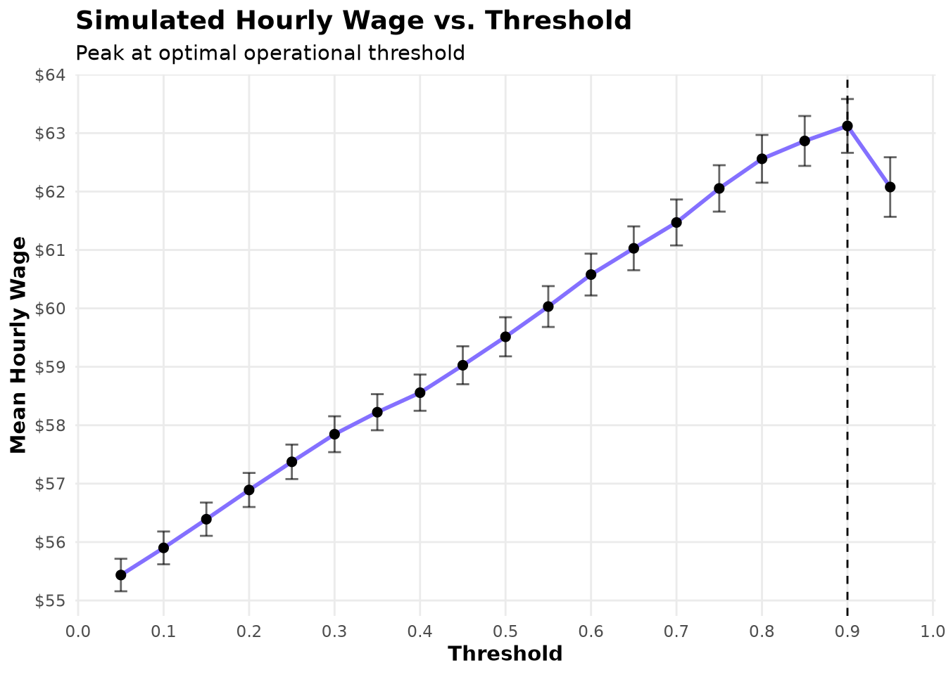
BestResult <- HourlyWageByTau[which.max(mean_wage), ]The results are striking. Contrary to the common intuition that drivers should “accept most trips and reject only the worst,” hourly wage increases monotonically with the threshold \(\tau\). It rises from $55.44 at \(\tau=0.05\) to $63.12 at \(\tau= 0.9\) — a 14.58% lift over the baseline of $55.09.
This counter-intuitive outcome is a powerful validation of the entire ADP pipeline. The lookahead-based labeling process (Chapter 5) created high-quality supervised targets that approximate the optimal short-horizon decision \(x_t^*\). The resulting PFA has learned subtle, high-value trip characteristics that the myopic baseline misses. By becoming more selective, the driver trades a modest increase in waiting time—already captured by the expanding-search logic—for substantially higher earnings per hour worked.
Show the code
ggplot(HourlyWageByTau, aes(tau_used, mean_wage)) +
  geom_vline(xintercept = BestResult$tau_used, linetype = 2) +
  geom_line(
    color = Params$ColorHighlight,
    linewidth = 1
  ) +
  geom_point(size = 2) +
  geom_errorbar(
    aes(ymin = mean_wage - 1.96 * se_wage, ymax = mean_wage + 1.96 * se_wage),
    width = 0.015,
    alpha = 0.6
  ) +
  scale_x_continuous(breaks = breaks_width(0.1)) +
  scale_y_continuous(breaks = breaks_width(1), label = dollar_format(1)) +
  labs(
    title = "Simulated Hourly Wage vs. Threshold",
    subtitle = "Peak at optimal operational threshold",
    x = "Threshold",
    y = "Mean Hourly Wage"
  ) +
  theme_minimal(base_family = Params$BaseFontFamily) +
  theme(
    legend.position = "none",
    plot.title = element_text(face = "bold", size = 14),
    axis.title = element_text(face = "bold"),
    panel.grid.minor = element_blank()
  )
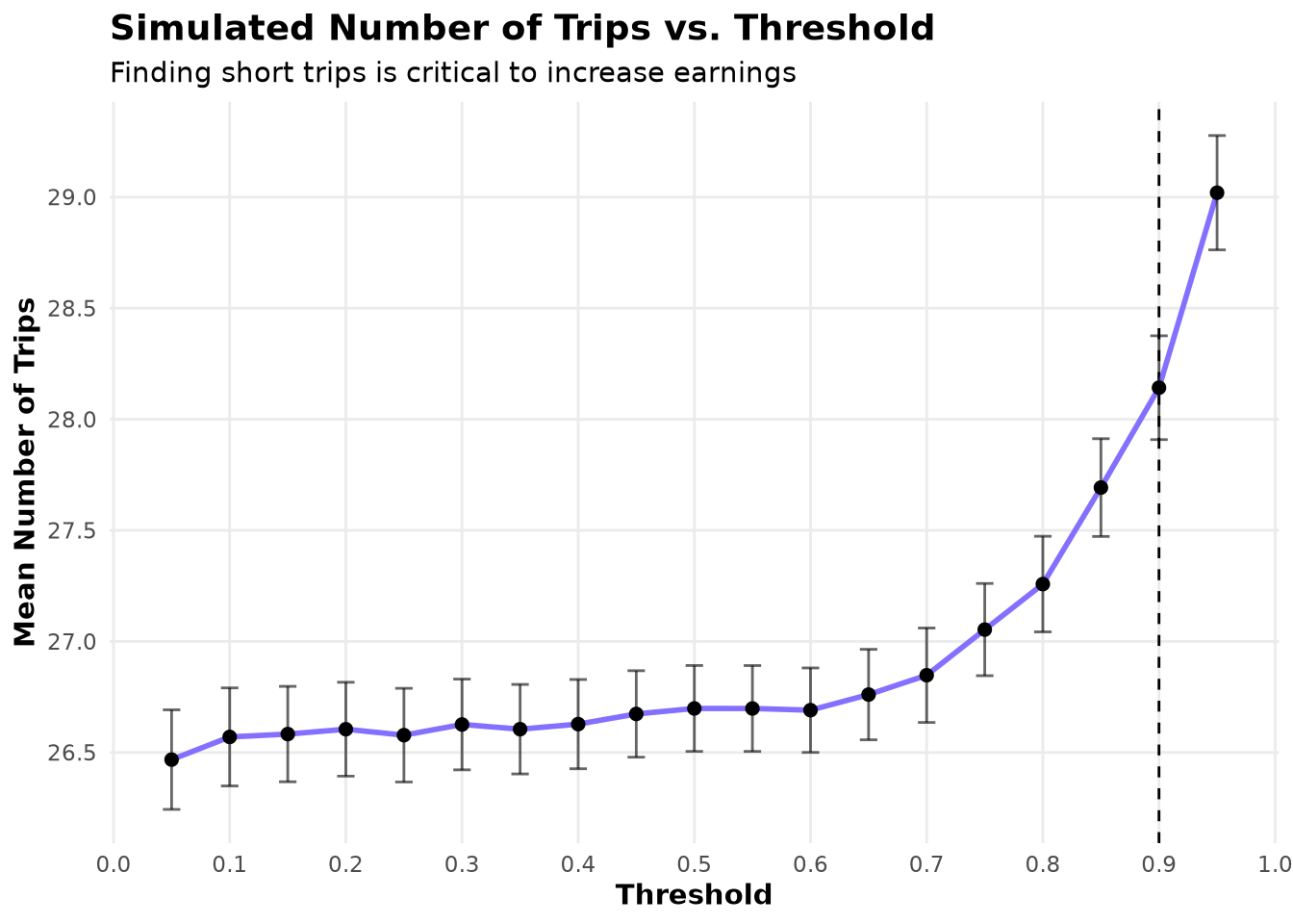
By exploring the average number of trips taken we see that, starting at \(\tau=0.7\), the number of trips increases. This indicates that the policy is successfully avoiding long, low-value trips, thereby freeing time for more short, high-value trips within the same working hours.
Show the code
ggplot(HourlyWageByTau, aes(tau_used, mean_n_trips)) +
  geom_vline(xintercept = BestResult$tau_used, linetype = 2) +
  geom_line(color = Params$ColorHighlight, linewidth = 1) +
  geom_point(size = 2) +
  geom_errorbar(
    aes(
      ymin = mean_n_trips - 1.96 * se_n_trips,
      ymax = mean_n_trips + 1.96 * se_n_trips
    ),
    width = 0.015,
    alpha = 0.6
  ) +
  scale_x_continuous(breaks = breaks_width(0.1)) +
  scale_y_continuous(breaks = breaks_width(0.5)) +
  labs(
    title = "Simulated Number of Trips vs. Threshold",
    subtitle = "Finding short trips is critical to increase earnings",
    x = "Threshold",
    y = "Mean Number of Trips"
  ) +
  theme_minimal(base_family = Params$BaseFontFamily) +
  theme(
    legend.position = "none",
    plot.title = element_text(face = "bold", size = 14),
    axis.title = element_text(face = "bold"),
    panel.grid.minor = element_blank()
  )
Warning
The simulation assumes abundant trip supply (“more passengers than taxis”). In reality, widespread selectivity could increase city-wide waiting times. Modeling supply-side dynamics remains an important direction for future work.
Final Policy Evaluation
We now re-run the simulator only at the optimal \(\tau^*\) using the exact same seeds as the baseline.
con <- dbConnect(duckdb(), dbdir = here("../NycTaxiBigFiles/my-db.duckdb"))

FinalPfaResults <- simulate_trips(
  con,
  SimulationStartDay,
  seeds = original_seeds,
  fitted_wf = XgboostFinalWorkflowTailorFitted,
  threshold = BestResult$tau_used
)

dbDisconnect(con, shutdown = TRUE)

pin_write(BoardLocal, FinalPfaResults, "FinalPfaResults", type = "qs2")
Note
This final run took approximately 2 days on the available hardware.
Computing the new hourly wage & CI
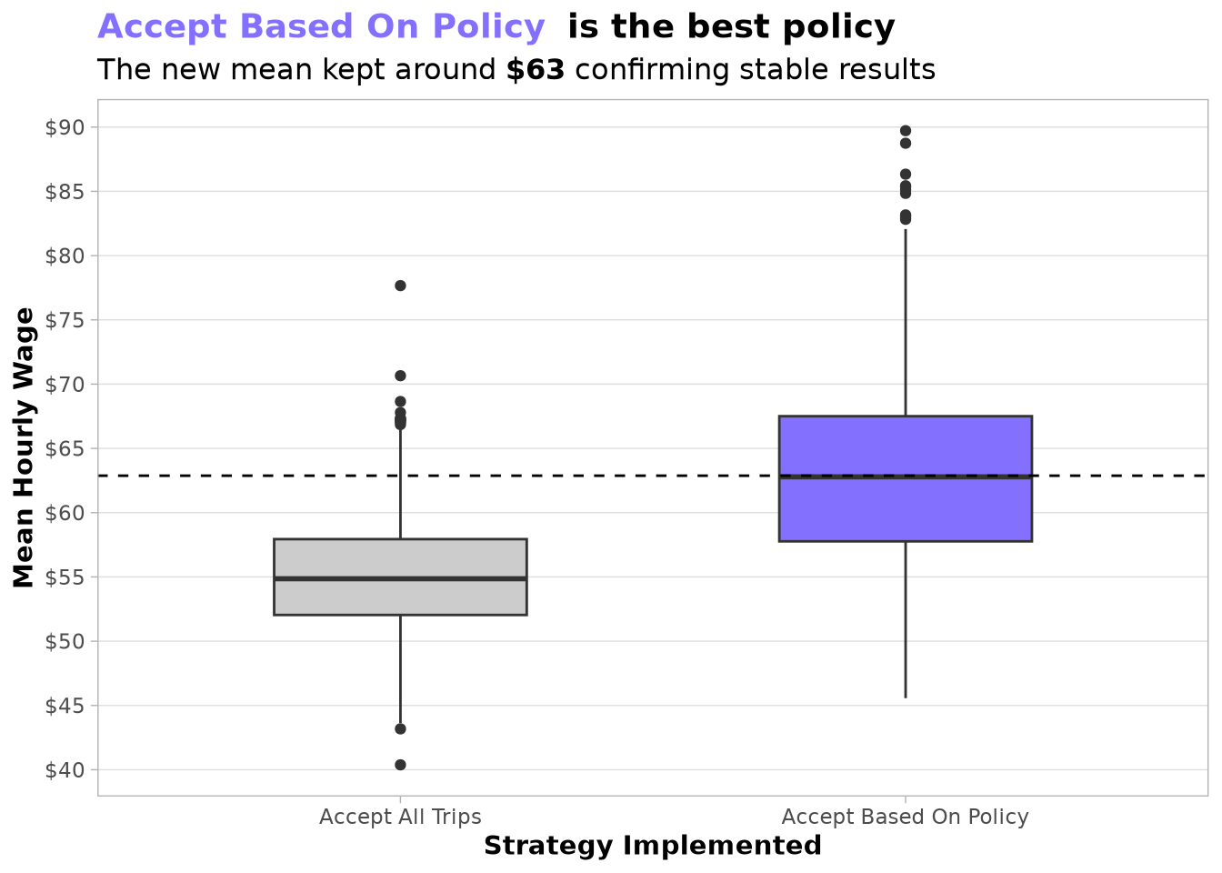
An important aspect visible in the new policy is its larger interquartile range. We expect this variability will be reduced once we add a strategic policy that selects the best starting zone and hour. We also anticipate that the second policy will help us reach the full 20 % lift targeted by the project.
The boxplot below confirms that the new mean hourly wage remained stable around the value obtained during grid search, demonstrating that the policy is robust and ready for production.
FinalPfaResults <- pin_read(BoardLocal, "FinalPfaResults")

PolicyLevels <- c("Accept All Trips", "Accept Based On Policy")

FinalPfaResultsSummary <- rbind(
  sim_start_trip_summary(SimulationHourlyWage, SimulationStartDay)[,
    strategy := PolicyLevels[1L]
  ],
  sim_start_trip_summary(FinalPfaResults, SimulationStartDay)[,
    strategy := PolicyLevels[2L]
  ],
  fill = FALSE
)

FinalPfaResultsSummary[, strategy := factor(strategy, PolicyLevels)]
Show the code
PolicyLevelsFillColors <- c(Params$ColorGray, Params$ColorHighlight)
setattr(PolicyLevelsFillColors, "names", PolicyLevels)

FinalPfaMeans <-
  FinalPfaResultsSummary[,
    .(daily_hourly_wage_mean = mean(daily_hourly_wage_mean)),
    keyby = "strategy"
  ][, setattr(daily_hourly_wage_mean, "names", as.character(strategy))]

ggplot(FinalPfaResultsSummary, aes(strategy, daily_hourly_wage_mean)) +
  geom_boxplot(aes(fill = strategy), width = 0.5) +
  geom_hline(yintercept = FinalPfaMeans[2L], linetype = 2) +
  scale_fill_manual(
    values = PolicyLevelsFillColors
  ) +
  scale_y_continuous(breaks = breaks_width(5), label = dollar_format(1)) +
  labs(
    title = paste0(
      "<span style='color:",
      Params$ColorHighlight,
      ";'>**",
      PolicyLevels[2L],
      "**</span> ",
      "**is the best policy**"
    ),
    subtitle = paste0(
      "The new mean kept around **",
      dollar(BestResult$mean_wage, accuracy = 1),
      "** confirming stable results"
    ),
    x = "Strategy Implemented",
    y = "Mean Hourly Wage"
  ) +
  theme_light(base_family = Params$BaseFontFamily) +
  theme(
    plot.title = element_markdown(size = 14, family = Params$BaseFontFamily),
    plot.subtitle = element_markdown(size = 12, family = Params$BaseFontFamily),
    axis.title = element_text(face = "bold"),
    panel.grid.major.x = element_blank(),
    panel.grid.minor.x = element_blank(),
    panel.grid.minor.y = element_blank(),
    legend.position = "none"
  )
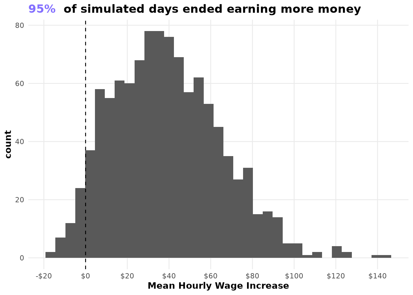
When we examine the improvement on a per-simulation-day basis, the gains are remarkably consistent: most simulated days earned more money after implementing the policy than using the original staregy.
Show the code
MeanPolicyDifference <- FinalPfaResultsSummary[,
  .(
    mean_difference = fifelse(
      strategy == PolicyLevels[1L],
      -daily_hourly_wage_mean,
      daily_hourly_wage_mean
    ) |>
      sum()
  ),
  by = "simulation_id"
]


InterceptToValidate <- 0

PropSimoOverIntercept <- MeanPolicyDifference[, mean(
  mean_difference >= InterceptToValidate
)]

ggplot(MeanPolicyDifference) +
  geom_histogram(aes(mean_difference), bins = 35) +
  geom_vline(xintercept = InterceptToValidate, linetype = 2) +
  scale_x_continuous(n.breaks = 10, label = dollar_format(1)) +
  labs(
    title = paste0(
      "<span style='color:",
      Params$ColorHighlight,
      ";'>**",
      percent(PropSimoOverIntercept, accuracy = 1),
      "**</span> ",
      "**of simulated days ended earning more money**"
    ),
    x = "Mean Hourly Wage Increase"
  ) +
  theme_minimal(base_family = Params$BaseFontFamily) +
  theme(
    plot.title = element_markdown(face = "bold", size = 14),
    panel.grid.minor = element_blank(),
    axis.title = element_text(face = "bold")
  )
Updating the probability threshold for production
Now that the simulation has identified the optimal operational threshold (\(\tau^* = 0.9\)), we can embed it directly into the final fitted workflow. This creates a production-ready model object that applies the exact decision rule we validated in the full-day Monte-Carlo simulator.
AcceptRejectPolicyFitted <-
  XgboostFinalWorkflowTailorFitted |>
  remove_tailor() |>
  add_tailor(tailor::adjust_probability_threshold(
    tailor::tailor(),
    BestResult$tau_used
  ))

pin_write(
  BoardLocal,
  AcceptRejectPolicyFitted,
  "AcceptRejectPolicyFitted",
  type = "qs2"
)
Key Takeaways
This chapter completes the ADP loop for the trip-acceptance policy. The combination of lookahead labeling, a well-calibrated PFA, and simulation-based threshold optimization has produced a practically usable, profit-driven decision rule that demonstrably outperforms the myopic baseline under the same uncertainty model.