Maximizing Driver Earnings by Selecting the Best Configuration and Time to Start
A Simulation-Driven Optimization of Ride-Hail Policies Using Tree-Based Interactions
Once we have a policy to decide if a trip should be taken or rejected, it is important to validate whether any of the following factors could cause an increase or decrease in taxi results:
Company
Start zone
Days of the week
Hour of the day
Defining Combinations to Simulate
As we have 196 zones to evaluate, 3 days to evaluate for each day of the week (7), 2 taxi companies, and we divide the day into 8 moments to measure (one every 3 hours), we end up with an experiment of 65,856 days to simulate.
Note
As DOLocationID is the variable used in the simulation to define the start zone of the first trip to simulate, we need to simulate all available zones for each combination.
Show the code
# Loading functions ----## To manage relative pathslibrary(here)library(pins)library(qs2)## Manipulate datalibrary(data.table)library(sf)library(DBI)library(duckdb)library(lubridate)library(timeDate)library(ggtext)library(scales)library(gt)## To run predictionslibrary(tidymodels)library(embed)library(themis)## Custom functions, board & paramsdevtools::load_all()BoardLocal <-board_folder(here("../NycTaxiPins/Board"))Params <- yaml::read_yaml(here("params.yml"))# Defining combinations ----## Getting shapes to useZonesShapes <-pin_read(BoardLocal, "ZonesShapes") |> (\(df) { df[ df[["borough"]] %chin%names(Params$BoroughColors), ] })() |>st_cast(to ="MULTIPOLYGON")setDT(ZonesShapes)ZonesShapes[, LocationID :=as.character(LocationID)]UniqueZoneIds <-unique(ZonesShapes$LocationID) |>sort()## Defining days to sampleYearDays <-data.table(days =seq.Date(make_date(2023), make_date(2023, 12, 31), by ="day"))YearDays[, wday := lubridate::wday(days)]set.seed(4879)SampledDays <- YearDays[, .SD[sample.int(.N, 3L)], by ="wday"]## Pre-build the big design matrix onceDataToSimulate <-CJ(DOLocationID = UniqueZoneIds,hvfhs_license_num =c("HV0003", "HV0005"),calendar_day =as.character(SampledDays$days),time_hour =seq(0, 21, length.out =8))DataToSimulate[, `:=`(trip_id =as.numeric(1:.N),request_datetime =paste(calendar_day, time_hour) |>ymd_h(),trip_time =0)]set.seed(4875)DataToSimulate |>slice_sample(n =8) |>gt() |># Add a title and subtitletab_header(title =md("**Situations to evaluate**"),subtitle =paste("A sample of the",comma(nrow(DataToSimulate)),"days to simulate" ) ) |># Format the date-time column nicelyfmt_datetime(columns = request_datetime,date_style ="iso",time_style ="hm" ) |># Left-align text, center numbers for better readabilitycols_align(align ="center",columns =everything() ) |># Give it a clean, modern themeopt_stylize(style =1, color ="gray")
Situations to evaluate
A sample of the 65,856 days to simulate
DOLocationID
hvfhs_license_num
calendar_day
time_hour
trip_id
request_datetime
trip_time
37
HV0005
2023-02-24
15
48230
2023-02-24 3:00 PM
0
125
HV0003
2023-07-03
6
7123
2023-07-03 6:00 AM
0
79
HV0003
2023-08-08
12
59565
2023-08-08 12:00 PM
0
236
HV0003
2023-11-01
15
38438
2023-11-01 3:00 PM
0
133
HV0005
2023-05-15
15
9958
2023-05-15 3:00 PM
0
125
HV0005
2023-05-15
12
7269
2023-05-15 12:00 PM
0
55
HV0003
2023-07-26
12
53173
2023-07-26 12:00 PM
0
82
HV0005
2023-12-08
6
60795
2023-12-08 6:00 AM
0
Running the Simulation
As I knew that running the whole process would take me several days, I decided to store the results of the simulations on disk for each zone. In this way, I was able to keep the experiment running as expected and stop the process between days to allow the computer to rest and reduce the risk of losing all progress. I also avoided memory problems while using the computer for daily activities.
To avoid the overhead of using an IDE, the next code was sourced from the terminal after connecting with ssh NycTaxi to consume as few resources as possible.
## Loading env# Getting prior policyAcceptRejectPolicyFitted <-pin_read(BoardLocal, "AcceptRejectPolicyFitted")# Competing renaming columnsDataToSimulate[, `:=`(calendar_day =NULL,time_hour =NULL,PULocationID ="1",wav_match_flag ="N",driver_pay =0,tips =0,dispatching_base_num ="",originating_base_num ="",on_scene_datetime = NA_POSIXct_,pickup_datetime = NA_POSIXct_,dropoff_datetime = NA_POSIXct_,trip_miles =0,base_passenger_fare =0,tolls =0,bcf =0,sales_tax =0,congestion_surcharge =0,airport_fee =0,shared_request_flag ="",shared_match_flag ="",access_a_ride_flag ="",wav_request_flag ="",month =1,year =2023,performance_per_hour =0)]# Check which zones are already doneAlreadyDone <-pin_list(BoardLocal) |>grep(pattern ="^InitialZoneSim_ZoneId_", value =TRUE) |>gsub(pattern ="InitialZoneSim_ZoneId_", replacement ="")zones_to_run <-setdiff(UniqueZoneIds, AlreadyDone)cat("→",length(zones_to_run),"zones left to simulate (out of",length(UniqueZoneIds),"total).\n")# === MAIN RESUMABLE LOOP ===for (zone_i in zones_to_run) {cat(" Simulating zone", zone_i, "... ")# Filter only this zone ZoneData <- DataToSimulate[list(zone_i), on ="DOLocationID"]# Fresh connection for each zone con <-dbConnect(duckdb(), dbdir =here("../NycTaxiBigFiles/my-db.duckdb")) ZoneSim <-simulate_trips( con, ZoneData,seeds =4878,fitted_wf = AcceptRejectPolicyFitted )dbDisconnect(con, shutdown =TRUE)# Save immediately with clear namepin_write( BoardLocal, ZoneSim,paste0("InitialZoneSim_ZoneId_", zone_i),type ="qs2" )cat("DONE (", nrow(ZoneSim), "rows)\n")}cat("✅ All zones simulated!\n")
Here is the list of zones simulated, and we can see that it took around 102 minutes to complete each zone, which means I invested around 14 days of computation to obtain the results below.
angelfeliz@debian:~/r-projects/NycTaxi$ ls -ld ../NycTaxiPins/Board/InitialZoneSim_ZoneId_*|wc-l196
Now we just need to summarize the results to start the exploration.
consolidate_all_simulations <-function(zone_id_data, board, sim_start_days) { consolidated_data =sim_start_trip_summary(pin_read(board, zone_id_data), sim_start_days )[, sim_start_days[, list(simulation_id = trip_id, hvfhs_license_num, DOLocationID,request_datetime =paste(calendar_day, time_hour) |>ymd_h() )][.SD, on ="simulation_id"], .SDcols =!patterns("_sd") ]return(consolidated_data)}InitialZoneSimResults <-pin_list(BoardLocal) |>grep(pattern ="^InitialZoneSim_ZoneId_", value =TRUE) |>lapply(FUN = consolidate_all_simulations,board = BoardLocal,sim_start_days = DataToSimulate ) |>rbindlist()# Adding region infoInitialZoneSimResults[ ZonesShapes, on =c("DOLocationID"="LocationID"),`:=`(borough = borough, start_zone_name = zone)]# Save immediately with clear namepin_write( BoardLocal, InitialZoneSimResults,"InitialZoneSimResults",type ="qs2")
Exploring Results
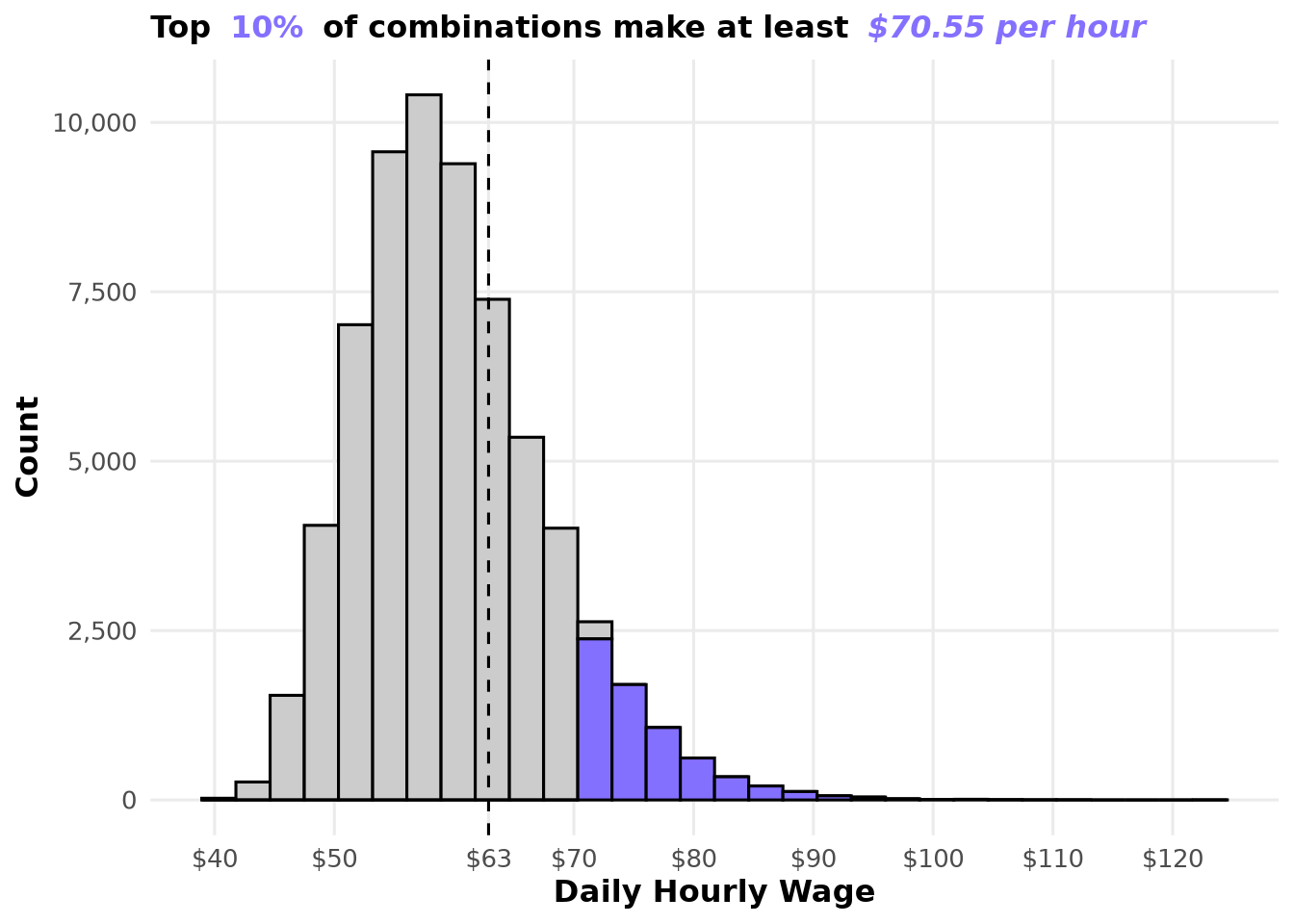
Before anything, it is important to confirm if changing the initial conditions of trips had an effect on the target variable. Just imagine that we see the same value for all combinations—we could stop the question simply by making the first chart.
But you can see in the following chart that there is a lot of variation. The data appears to follow a log-normal distribution due to its long right tail. These are really promising results. The goal behind this experiment is to identify the starting configurations that can beat the current baseline of $55.09, and it is clear based on the chart that the top 10% present higher daily hourly wages than the baseline.
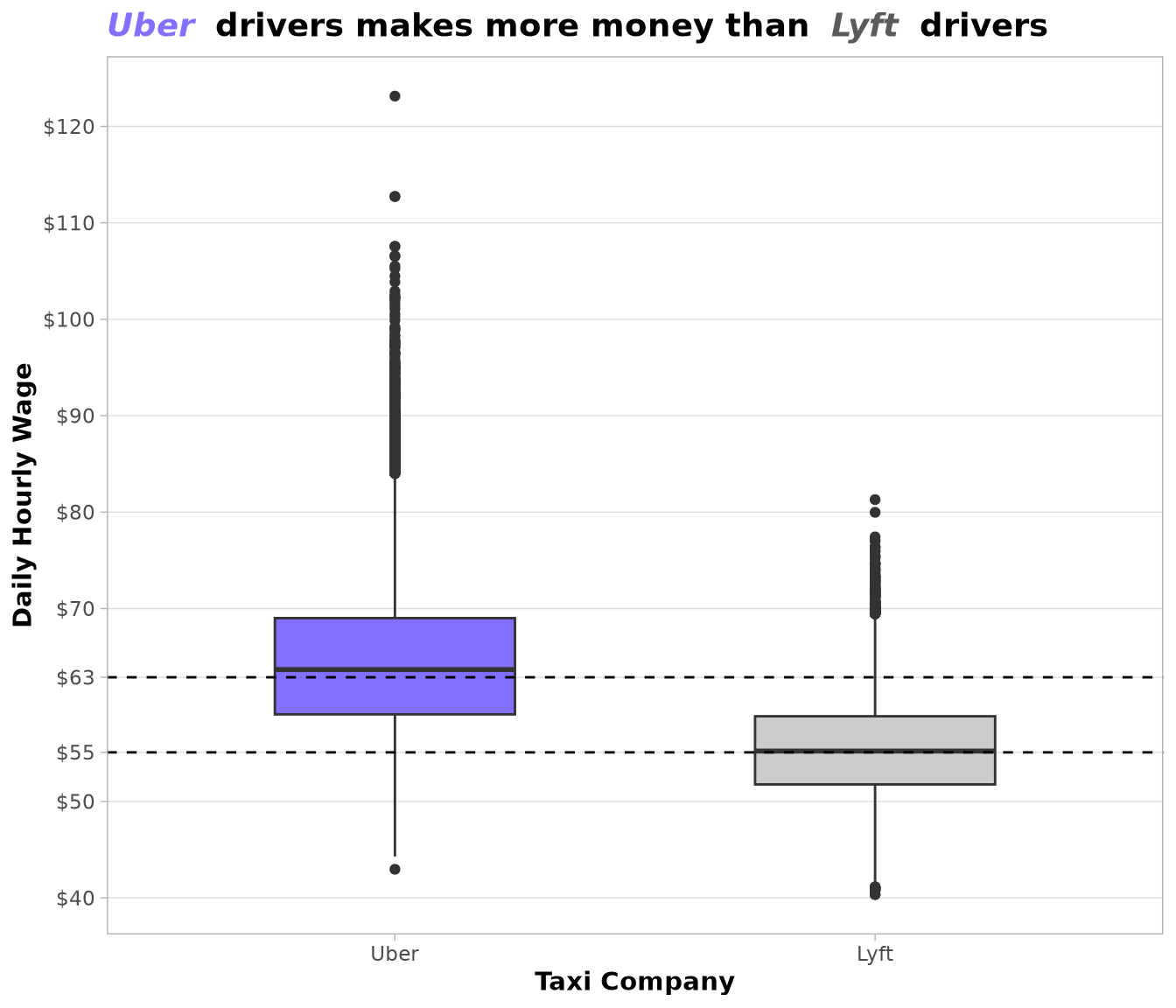
As we can see, the improvement behind the policy only benefits Uber drivers, as the median hourly wage for Lyft drivers matches the exact value of the baseline. As a result, our policy will always recommend Uber as the taxi company.
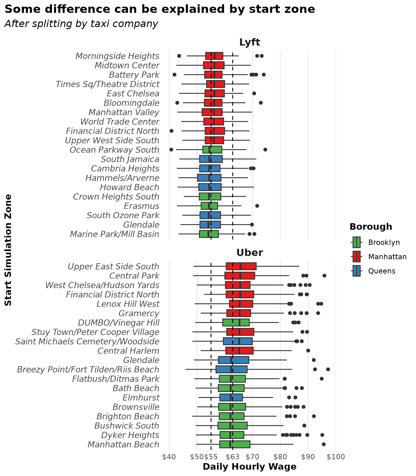
After isolating the effect of the taxi company on the hourly wage, we can see by selecting the zones with the highest and lowest medians that the change in the target variable explained by starting zone is low. We are evaluating 196 zones, and the increase in the median for Uber drivers was only $2 over the baseline ($62.88) after implementing the trip selection model. Based on the boxplot, we can conclude that zones do not provide enough information to explain the variance present in the target variable.
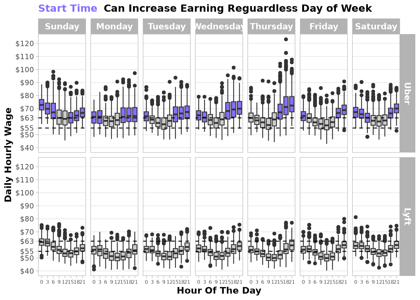
Based on the next chart, we can see a strong effect of start hour on the target variable and some moderate interactions with the day of the week. The hourly wage is higher at 0 hours on Sundays and Saturdays, but those increases are not present on weekdays.
Based on the prior exploration, it is clear that the most important rule found so far is to choose Uber as the company. However, to improve earnings further, we need to find better interactions between variables. For that reason, we are going to start with a tree model to see if the model can find the most important interactions to explain changes in the target variable.
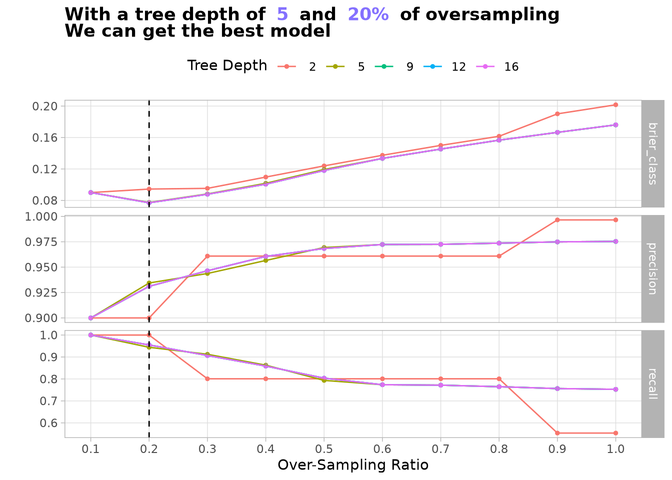
To tune the model, we know that the most important hyperparameter is tree_depth to limit how many splits the tree can make, which controls vertical complexity. As a result, we want to use the minimum value possible.
Since we have a lot of data to explore due to the number of zones in the experiment, we know that min_n—which sets the minimum number of data points required in a node to allow a further split—will not be an important hyperparameter, as most splits will have many data points to avoid overfitting.
To help the tree find the important patterns, we apply the following transformations to the original data:
As start_zone presents high cardinality, we substitute it with hourly_wage_mean_by_zone after isolating the effect of taxi company.
To allow the model to see hour of the day and time of the week as the cycles they represent in real life—where the same time repeats every 24 hours and the same time in the week repeats every 168 hours—we create the variables day_cycle_sin_1 and day_cycle_cos_1 instead of just using time_hour, and week_cycle_sin_1 and week_cycle_cos_1 instead of using the original week_day.
We show taxi_company as a boolean variable to keep all variables numeric.
DecisionTreeRecipe <-recipe( is_top_trip ~ hvfhs_license_num + DOLocationID + request_datetime + simulation_id + daily_hourly_wage_mean,data = InitialZoneSimResults) |># Creating variables to use laterstep_mutate(taxi_company =ifelse(hvfhs_license_num =='HV0003', "Uber", "Lyft") |>factor(levels =c("Lyft", "Uber")),day_cycle =hour(request_datetime),week_cycle = (wday(request_datetime) -1) *24+ day_cycle,hourly_wage_mean_by_zone =paste0(DOLocationID, "-", taxi_company) ) |># Changing zones with their meanstep_lencode( hourly_wage_mean_by_zone,outcome =vars(daily_hourly_wage_mean),smooth =FALSE ) |># Transforming company to binary variablestep_dummy(taxi_company) |># Creating Cyclesstep_harmonic( day_cycle,cycle_size =24,frequency =1,keep_original_cols =FALSE ) |>step_harmonic( week_cycle,cycle_size =168,frequency =1,keep_original_cols =FALSE ) |># Saving original varsupdate_role( simulation_id, DOLocationID, daily_hourly_wage_mean, hvfhs_license_num, request_datetime,new_role ="additional info" ) |># Removing original variablesstep_upsample(is_top_trip, over_ratio =tune("over_ratio"))
Now, after all this configuration, we are ready to consolidate all that logic into a compact workflow that will help us fit and evaluate our model using all tools from tidymodels.
As this is a simple model and we just need to tune 2 parameters, we can use the grid method to find the best trip possible with 10-fold cross-validation to estimate the model error without taking testing data. We just need to understand the results of the experiment rather than using this model to make predictions.
After all this exploration, we not only need to take the configuration that better predicts the results, but instead the one that loses less prediction power without moving too high in tree_depth. For that reason, rather than using the default function select_best, we use a different version that is more flexible in the brier_class score to select the configuration with less model complexity, as we want a model that is easy to explain.
autoplot(DecisionTreeWfTuned) +geom_vline(xintercept = DecisionTreeWfBestConfig$over_ratio, linetype =2) +scale_x_continuous(breaks =breaks_width(0.1)) +labs(title =paste0("**With a tree depth of**",highlight_text(DecisionTreeWfBestConfig$tree_depth),"**and**", DecisionTreeWfBestConfig$over_ratio |> scales::percent() |>highlight_text(),"**of oversampling**<br>**We can get the best model**" ) ) +theme_light(base_family = Params$BaseFontFamily) +theme(legend.position ="top",plot.title =element_markdown(family = Params$BaseFontFamily),plot.subtitle =element_text(family = Params$BaseFontFamily,face ="italic" ),legend.title =element_markdown(family = Params$BaseFontFamily),panel.grid.minor =element_blank() )
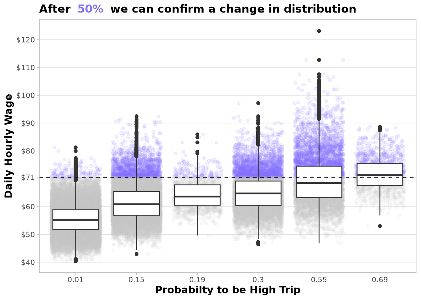
Now we are ready to train the model and see the probabilities predicted by the model. The results are really good, as we can see that the median of daily_hourly_wage_mean increases with the probability of the trip being of high value.
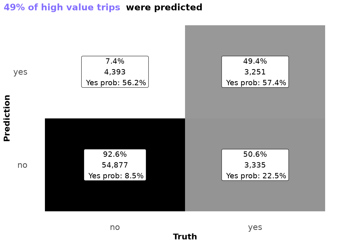
I feel really good about the results provided in the confusion matrix, as the model was able to predict 41% of days as high value and only incorrectly predicted high-value trips for 5% of all possible trips—a solid pattern.
To facilitate the interpretation of the effect of using the tree model to change the behavior of the taxi driver, we will range all variables from 0 to 1 in order to have the model coefficients in dollars per hour.
As we want to define the effect of using the tree model on the hourly mean wage of drivers, it is really important to confirm that the variables used to train the model do not present collinearity. Based on the table, it is clear that taxi_company_Uber and hourly_wage_mean_by_zone are contributing the same information. As a result, we know that hourly_wage_mean_by_zone is just dividing drivers by company, and the zone is not providing any additional information.
Show the code
linear_reg() |>set_engine("lm") |>fit(data = TreeResultsToExplore,formula = daily_hourly_wage_mean ~ tree_model_high_value + hourly_wage_mean_by_zone + taxi_company_Uber + day_cycle_sin_1 + day_cycle_cos_1 + week_cycle_sin_1 + week_cycle_cos_1 ) |>extract_fit_engine() |> car::vif() |>round(digits =2) |> (\(x) tibble(variable =names(x), vif = x))() |>arrange(desc(vif)) |>gt() |>tab_header(title ="Multicollinearity Diagnostic: Variance Inflation Factor (VIF)",subtitle ="Checking stability of factors determining hourly income" ) |>cols_label(variable ="Variable",vif ="VIF Score" ) |># Format VIF to 2 decimal placesfmt_number(columns = vif, decimals =2) |># Style variable names to be italicizedtab_style(style =cell_text(style ="italic"),locations =cells_body(columns = variable) ) |># Add a visual warning for high multicollinearity (VIF > 5 or 10)tab_style(style =cell_text(color ="darkred", weight ="bold"),locations =cells_body(columns =everything(), rows = vif >=5.0) ) |>tab_source_note(source_note ="Note: VIF > 5 indicates potential multicollinearity issues that may inflate standard errors." )
Checking stability of factors determining hourly income
Variable
VIF Score
taxi_company_Uber
45.38
hourly_wage_mean_by_zone
45.21
tree_model_high_value
1.27
day_cycle_sin_1
1.08
day_cycle_cos_1
1.01
week_cycle_cos_1
1.01
week_cycle_sin_1
1.00
Note: VIF > 5 indicates potential multicollinearity issues that may inflate standard errors.
With 65,856 simulated days all coefficients are statistically significant, so the focus should be on the magnitude of each effect.
The regression reveals a clear hierarchy of factors:
A driver that use Uber can earn up to $7.71 more per hour compared to a driver that use Lyft.
Starting at a favorable time of day can add up to $5.52 per hour (captured by day_cycle_cos_1), while an unfavorable hour can subtract up to $2.33.
Day-of-week effects are small (under $1.58 in either direction), confirming that what time of day the driver starts matters far more than which day of the week they work.
A driver who follows the tree model’s accept/reject strategy earns an additional $5.81 per hour on top of all the above. This reflects the specific company-and-timing combinations the tree identified as high-value that no single variable captures independently.
In practice, a driver making all the right decisions — starting with Uber at a favorable time and following the tree model’s strategy — can move from the baseline of $54/hour to approximately $70/hour, representing a 34% improvement in hourly earnings.
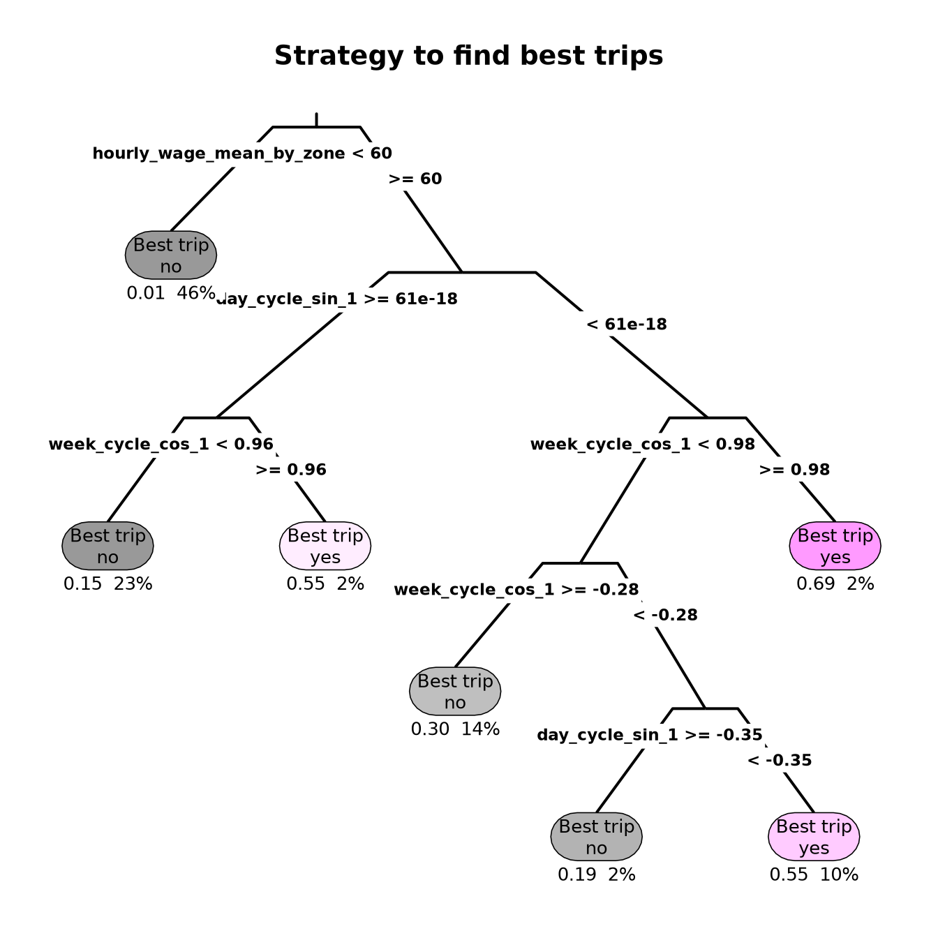
As the most important variable for the model was hourly_wage_mean_by_zone, let’s explore which zones were excluded by the model. As a first step, we can extract the split used for that variable.
As the variables used by the model are not easy to interpret by humans, let’s integrate into a single dataframe the features used by the model, the features before using the recipe transformations, and the predictions of the model to create visuals that translate what was learned by the model.
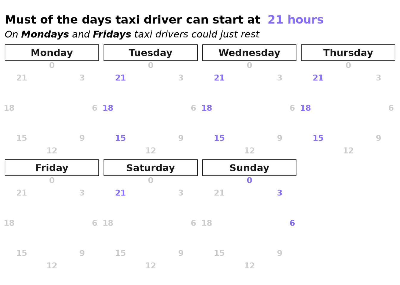
ValidHoursToStartWorking <-pin_read(BoardLocal, "ValidHoursToStartWorking")ValidHoursToStartWorking |>gt() |># Add a title and subtitletab_header(title =md("**Valid Hour To Use**"),subtitle ="In case that of low value start times" ) |># Left-align text, center numbers for better readabilitycols_align(align ="center",columns =everything() ) |># Give it a clean, modern themeopt_stylize(style =1, color ="gray")
Valid Hour To Use
In case that of low value start times
hour
week_day
week_cycle
0
1
0
3
1
3
6
1
6
15
3
63
18
3
66
21
3
69
15
4
87
18
4
90
21
4
93
15
5
111
18
5
114
21
5
117
21
7
165
All this logic was implemented in the optimize_trip_start_time function, and we can make sure that the trips fill these conditions after applying the function over the trips used to create the baseline.
list(SimulationStartDay, SimulationStartDayUpdated) |>lapply(\(dt) { dt[,list(Uber_prop =mean(hvfhs_license_num =="HV0003"), N = .N), by =list(week_day =factor( Weekdays[wday(request_datetime)],levels =c(Weekdays[-1L], Weekdays[1L]) ) ) ] }) |>c(list(by ="week_day",all =TRUE,suffixes =c("_original", "_updated") )) |>do.call(what ="merge" ) |>gt() |># Header & Titlestab_header(title ="Simulation Start Days After Policy",subtitle ="Now all days are with Uber and any day starts on Monday or Friday" ) |># Apply styling to Header (Dark Blue/Gray theme from your style)tab_style(style =cell_text(color ="white", weight ="bold"),locations =cells_title() ) |>tab_style(style =cell_fill(color ="#2c3e50"),locations =cells_title() ) |># Format Proportions (Percentages look great here, or use decimals = 4 to match your preference)fmt_percent(columns =c(Uber_prop_original, Uber_prop_updated),decimals =0 ) |># Format Counts (Integers)fmt_integer(columns =c(N_original, N_updated) ) |># Handle Missing Values (Replaces NA with a clean em-dash)sub_missing(columns =everything(),missing_text ="—" ) |># Group columns visually using spannerstab_spanner(label ="ORIGINAL CONDITIONS",columns =c(Uber_prop_original, N_original) ) |>tab_spanner(label ="UPDATED CONDITIONS",columns =c(Uber_prop_updated, N_updated) ) |># Clean Column Labelscols_label(week_day ="DAY OF WEEK",Uber_prop_original ="UBER PROP.",N_original ="N",Uber_prop_updated ="UBER PROP.",N_updated ="N" ) |># Alignmentcols_align(align ="left",columns = week_day ) |># General Table Optionstab_options(table.font.names ="Arial",table.background.color ="white",column_labels.font.weight ="bold",column_labels.background.color ="#f8f9fa",table.width =pct(100),quarto.disable_processing =TRUE )
Simulation Start Days After Policy
Now all days are with Uber and any day starts on Monday or Friday
DAY OF WEEK
ORIGINAL CONDITIONS
UPDATED CONDITIONS
UBER PROP.
N
UBER PROP.
N
Monday
69%
140
—
—
Tuesday
68%
120
100%
384
Wednesday
71%
144
100%
142
Thursday
73%
152
100%
154
Friday
72%
161
—
—
Saturday
75%
178
100%
345
Sunday
78%
166
100%
36
Evaluating the Policy
To evaluate this policy under the same conditions we evaluated the baseline and the accept/reject policy, we are using the same simulation with the difference that now we are passing the start_day_fitted_model and valid_start_times_dt arguments, which will be used by optimize_trip_start_time to change the initial conditions of each day.
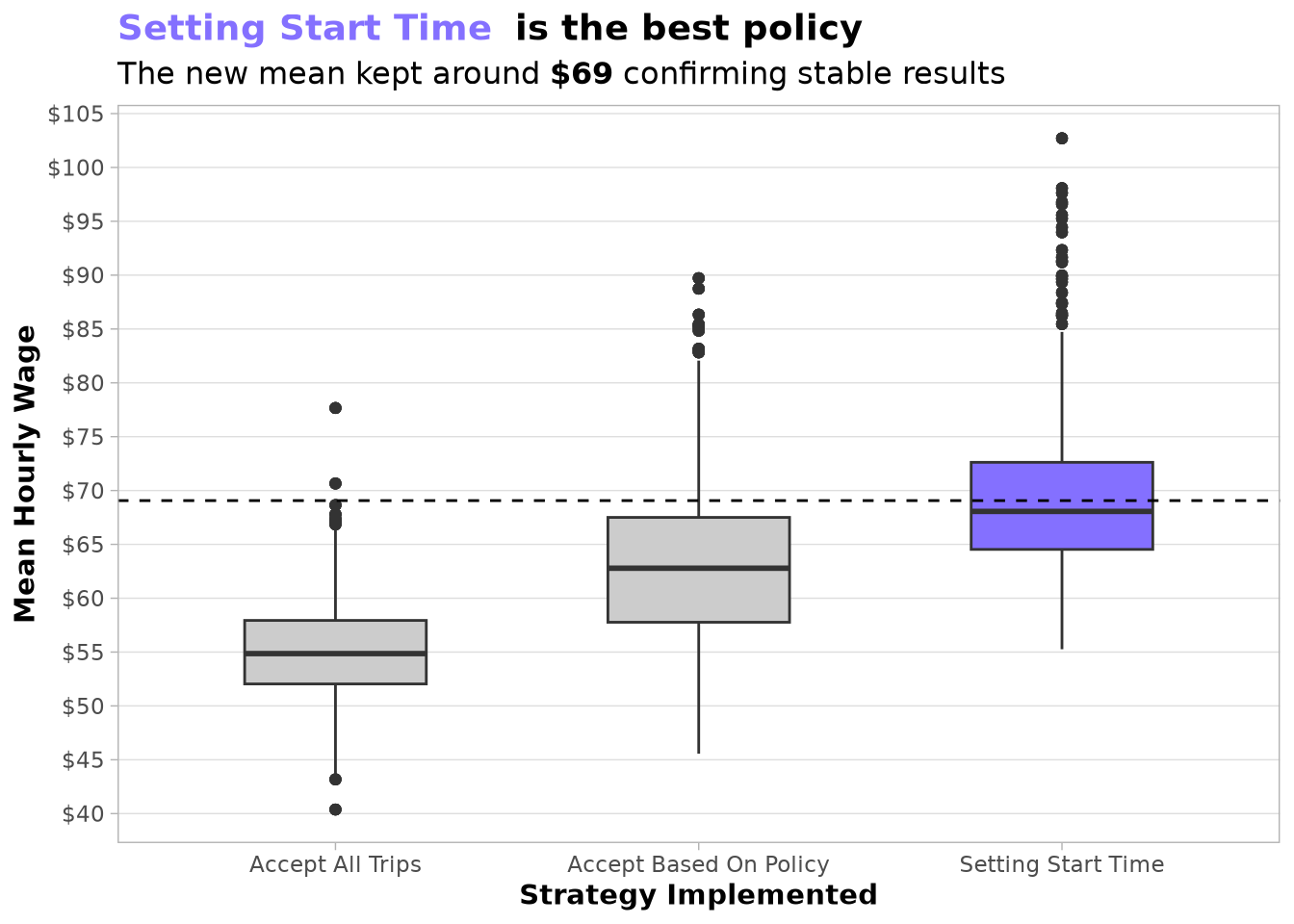
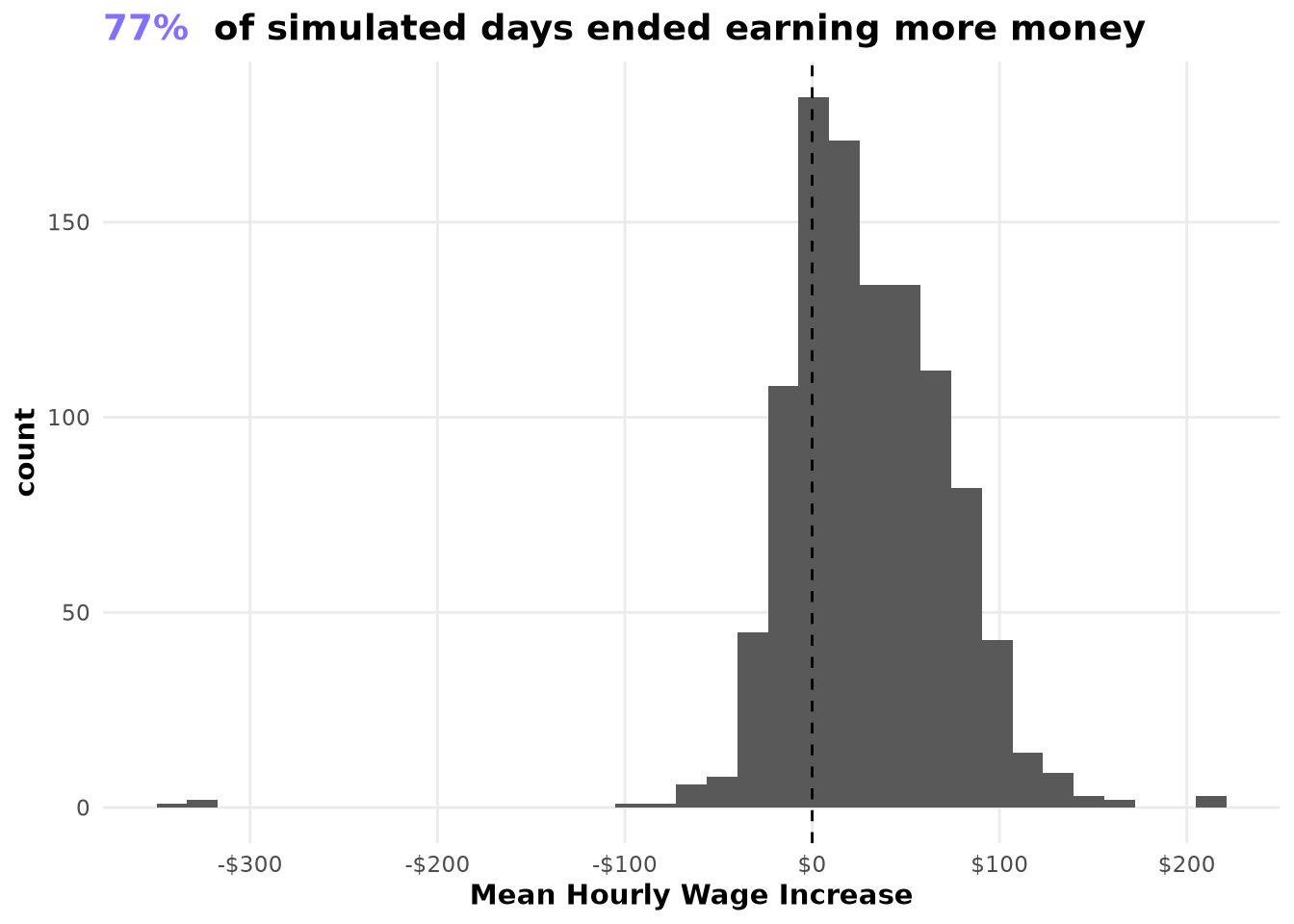
The results are amazing: we move from having $55.09 per hour to being able to earn on average $69.07 if we implement both policies at the same time. We can also see that the chart presents outliers of days that ended earning more than $90, which was not possible even using the accept/reject policy alone.
If we compare the difference between the accept/reject policy and the policy created now to start the trips, we can confirm that the increase in the average is not due to an increase in variability but rather because in the majority of cases the taxi drivers are getting better results than in the original situation.
Platform Selection: Drivers should exclusively choose Uber. The selective trip policy provides no benefits for Lyft, whose median wage stagnates at the $55.09 baseline , whereas driving for Uber adds up to +$7.71/hour.
Geographic Zones: Initial start zones have a negligible impact (only a $2 variance over the baseline). Due to severe multicollinearity with the choice of company, geographic start zones provide no useful independent information.
Shift Timing: Favorable starting hours (especially night shifts) add up to +$5.52/hour , while unfavorable starting times subtract up to -$2.33/hour.
Day of the Week: Day-of-the-week variance is minor (under $1.58 in either direction) ; however, the optimized policy explicitly excludes Mondays and Fridays as sub-optimal working days.
Final Policy Lift: Pairing the trip-acceptance policy with the strategic “Setting Start Time” configuration boosts average hourly wages from $55.09 to $69.07 , while unlocking exceptional high-yield outlier days exceeding $90/hour.