# Helper packages for data wrangling and awesome plotting
library(dplyr)
library(recipes)
library(ggplot2)

# Modeling packages for fitting MARS models
# and automating the tuning process
library(earth)
library(caret)
library(rsample)
library(parsnip)

# Model interpretability packages
# for variable importance and relationships
library(vip)
library(pdp)7 Non-parametric Methods
7.1 Smoothing splines
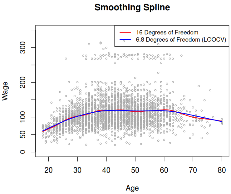
They arise as a result of minimizing a residual sum of squares criterion subject to a smoothness penalty.
In this method rather than trying to minimize \(\text{RSS} = \sum_{i=1}^n (y_i - g(x_i))^2\), we try to find a function \(g(x)\), known as smoothing spline, which could minimize the following expression based on the \(\lambda\) nonnegative tuning parameter.
\[ \underbrace{\sum_{i=1}^n (y_i - g(x_i))^2 }_{\text{loss function (data fitting)}} + \underbrace{\lambda \int g''(t)^2dt}_{\text{penalty term (g varibility)}} \]
The second derivative of \(g(t)\) measure how wiggly is the function near \(t\), where its value is \(0\) when the function is a straight line as a line is perfectly smooth. The we can use integral to get total change in the function \(g'(t)\), over its entire range. As consequence, the larger the value of \(\mathbf{\lambda}\) , the smoother \(\mathbf{g}\) will be.
The function \(g(x)\) is a natural cubic spline with knots at \(x_1, \dots ,x_n\). As results the effective degrees of freedom (\(df_{\lambda} = \sum_{i=1}^n \{ \mathbf{S}_{\lambda} \}_{ii}\)) are between \(n\) and \(2\) depending on the value of \(\mathbf{\lambda}\).
We can use cross-validation to find the best value which can minimize the RSS. It turns out that the leave one-out cross-validation error (LOOCV) can be computed very efficiently for smoothing splines, with essentially the same cost as computing a single fit, using the following formula:
\[ \text{RSS}_{cv} (\lambda) = \sum_{i = 1}^n (y_i - \hat{g}_\lambda^{(-i)} (x_i))^2 = \sum_{i = 1}^n \left[ \frac{y_i - \hat{g}_{\lambda} (x_i)} {1 - \{ \mathbf{S_{\lambda}} \}_{ii}} \right]^2 \]
Where:
- \(\hat{g}_\lambda^{(-i)}\): Refers to the function fitted without the ith observation \((x_i, y_i)\).
- \(\hat{g}_\lambda\): Refers the smoothing spline function fitted to all of the training observations.
7.2 Local regression
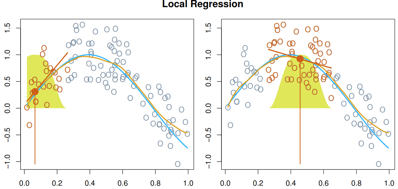
Computes the fit at target point \(x_0\) using only the nearly training observations by:
- Gather the \(s=k/n\) closest (known as span) fraction of points. This step is very important as it controls the flexibility level can be selected using cross-validation*.
- Assign a weight \(K_{i0} = K(x_i, x_0)\) for each selected point based on the distance to \(x_0\). As lower is the distance as higher needs to be the weight.
- Find the coefficients which minimize the weighted least squares regression for the current \(x_0\) value.
\[ \sum_{i=1}^n = K_{i0}(y_i - \beta_0 - \beta_1x_i)^2 \]
- Calculate the fitted value of \(x_0\) using \(\hat{f}(x_0) = \hat{\beta}_0 + \hat{\beta}_1x_0\).
In the next illustration we can see how the model works with some simulated data.
It performs poorly when we have more than 3 or 4 predictors in our model.
7.3 Multivariate Adaptive Regression Splines (MARS)
| Lineal models | Nonlinear models |
|---|---|
| If you know a priori the nature of a nonlinear relation you could manually adapt the model to take in consideration the nonlinear patters by including polynomial terms or step functions | The model would find the important nonlinear interactions present in the data |
7.3.1 Extending linear models
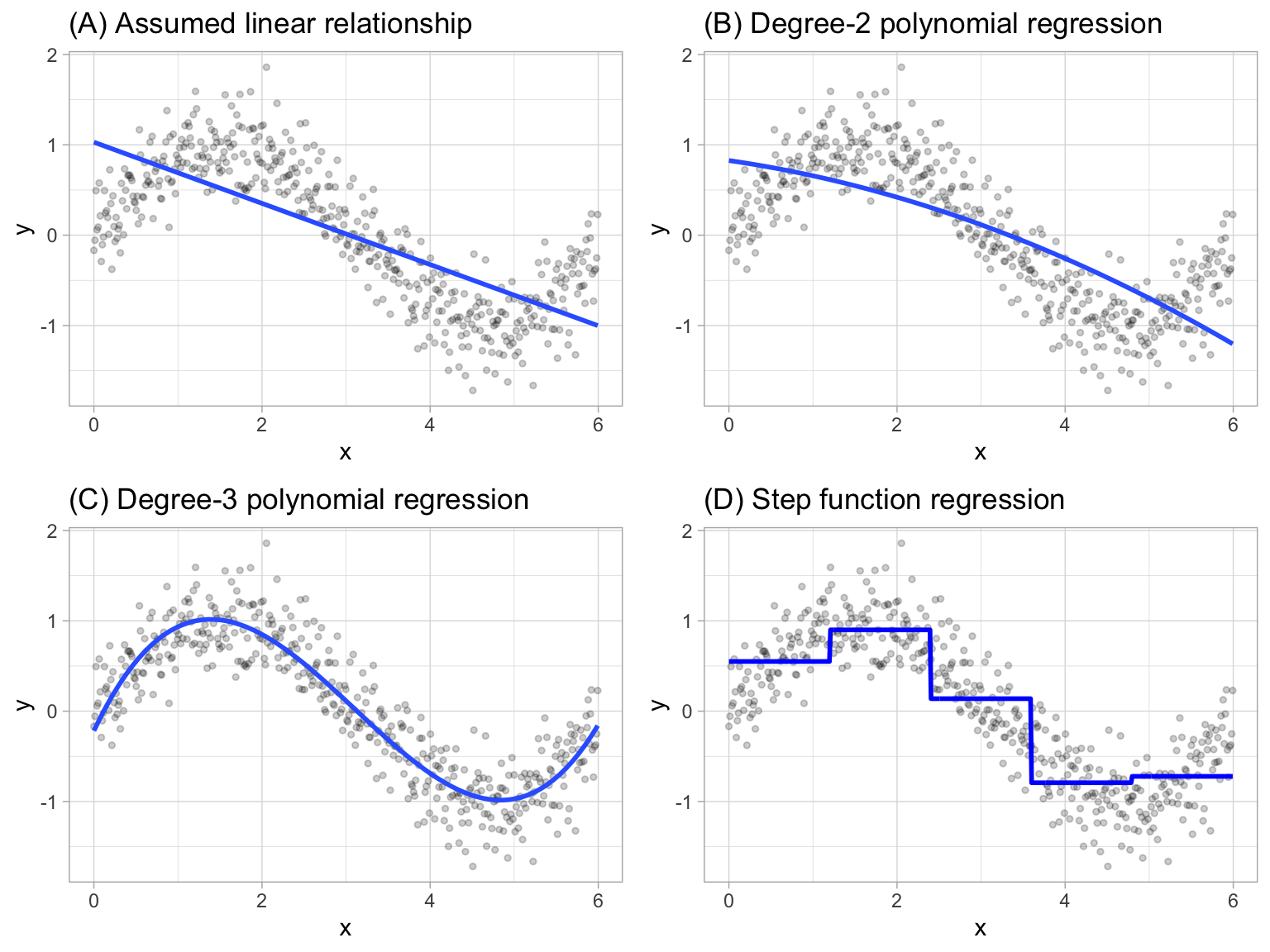
- Polynomial regression: It extends the linear model by adding extra predictors, obtained by raising each of the original predictors to a power. Generally speaking, it is unusual to use \(d\) greater than 3 or 4 as the larger \(d\) becomes, the easier the function fit becomes overly flexible and oddly shaped as it tends to increase the presence of multicollinearity.
\[ y_i = \beta_0 + \beta_1 x_i + \beta_2 x_i^2 + \beta_3 x_i^3 + \dots + \beta_d x_i^d + \epsilon_i \]
- Piecewise constant regression: It’s a step function which breaks the range of \(X\) into bins and fit a simple constant (e.g., the mean response) in each bin.
If we define the cutpoints as \(c_1, c_2, \dots, c_K\) in the range of X, we can create dummy variables to represent each range. For example, if \(c_1 \leq x_i < c_2\) is TRUE then \(C_1(x_i) = 1\) and then we need to repeat that process for each value of \(X\) and range. As result we can fit a lineal regression based on the new variables.
\[ y_i = \beta_0 + \beta_1 C_1(x_i) + \beta_2 C_2(x_i) \dots + \beta_K C_K(x_i) + \epsilon_i \]
7.3.2 Explaning the model
MARS is an algorithm that automatically creates a piecewise linear model after grasping the concept of multiple linear regression.
It will first look for the single point across the range of \(X\) values where two different linear relationships between \(Y\) and \(X\) achieve the smallest error (e.g., Sum of Squares Error). What results is known as a hinge function \(h(x-a)\), where \(a\) is the cutpoint value (knot).
For example, let’s use \(1.183606\) the our first knot.
\[ y = \begin{cases} \beta_0 + \beta_1(1.183606 - x) & x < 1.183606, \\ \beta_0 + \beta_1(x - 1.183606) & x < 1.183606 \\ \end{cases} \]
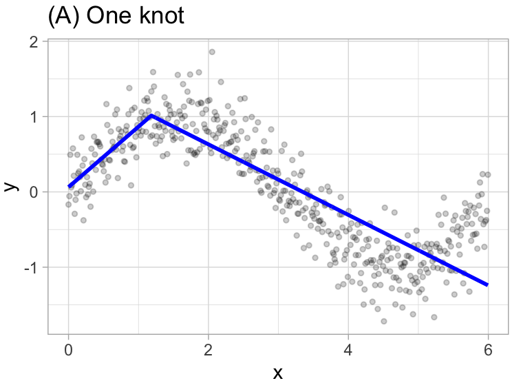
Once the first knot has been found, the search continues for a second knot.
\[ y = \begin{cases} \beta_0 + \beta_1(1.183606 - x) & x < 1.183606, \\ \beta_0 + \beta_1(x - 1.183606) & x < 1.183606 \quad \& \quad x < 4.898114 \\ \beta_0 + \beta_1(4.898114 - x) & x > 4.898114 \end{cases} \]
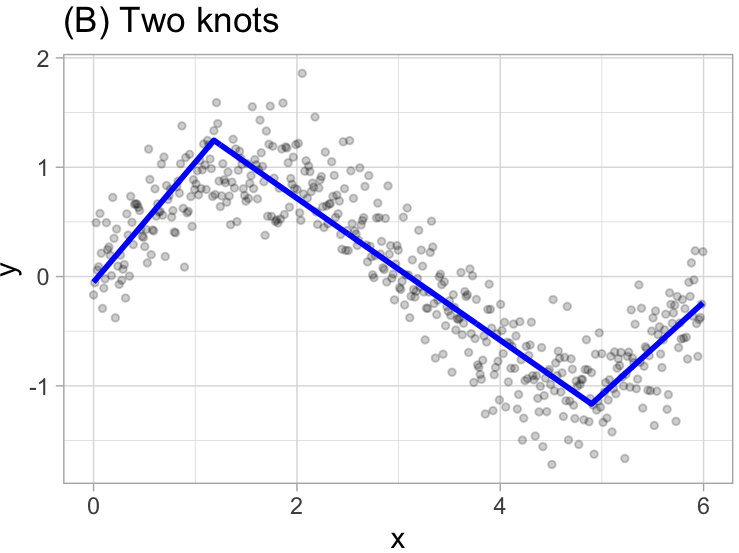
This procedure continues until \(R^2\) change by less than 0.001.
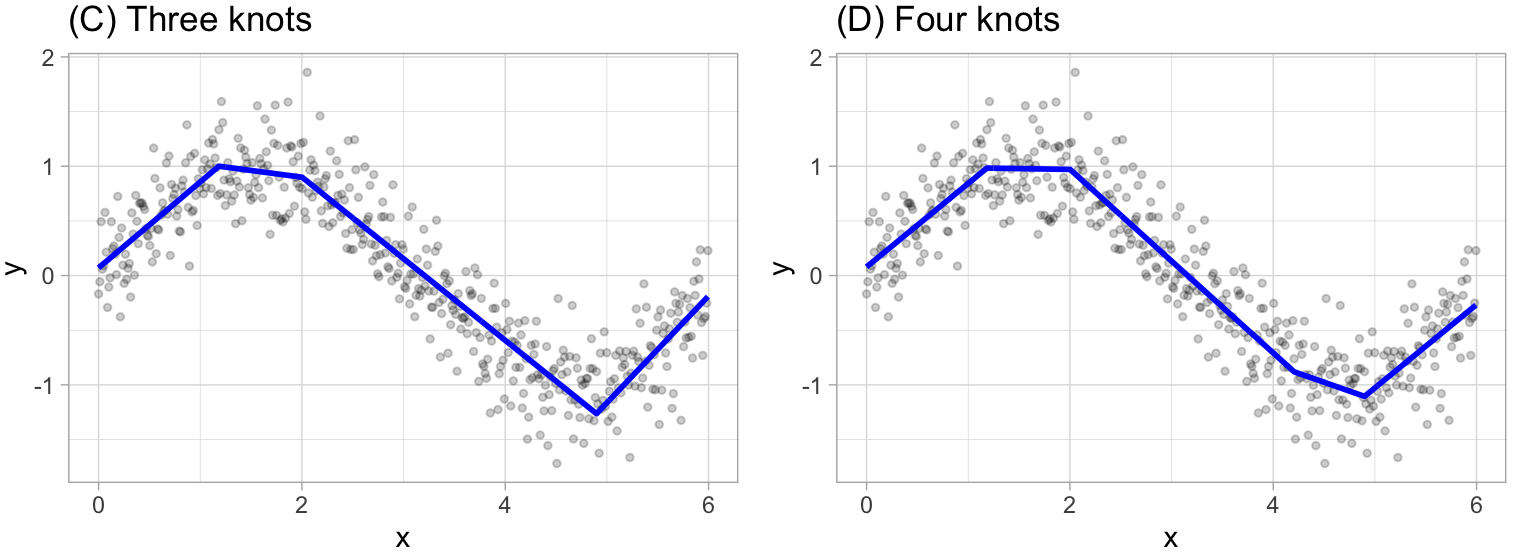
Then the model starts the pruning process, which consist in using cross-validation to remove knots that do not contribute significantly to predictive accuracy. To be more specific the package used in R performs a Generalized cross-validation which is a shortcut for linear models that produces an approximate leave-one-out cross-validation error metric.
7.3.3 Loading prerequisites
We can fit a direct engine MARS model with the earth (Enhanced Adaptive Regression Through Hinges) package, as “MARS” is trademarked and licensed exclusively to Salford Systems and cannot be used for competing software solutions.
Libraries to use
Data to use
set.seed(123)

ames_split <-
  initial_split(
    AmesHousing::make_ames(),
    prop = 0.7,
    strata = "Sale_Price"
  )

ames_train  <- training(ames_split)
ames_test   <- testing(ames_split)
7.3.4 Explaning model’s summary
Let’s explain the summary of a trained model.
mars1 <-
  earth(Sale_Price ~ ., data = ames_train)

mars1
Selected 41 of 45 terms, and 29 of 308 predictors
Termination condition: RSq changed by less than 0.001 at 45 terms
Importance: Gr_Liv_Area, Year_Built, Total_Bsmt_SF, ...
Number of terms at each degree of interaction: 1 40 (additive model)
GCV 511589986 RSS 967008439675 GRSq 0.9207836 RSq 0.9268516- The number of terms correspond to the number of coefficients used by the model.
                        Sale_Price
(Intercept)           227597.23167
h(Gr_Liv_Area-3194)     -287.99337
h(3194-Gr_Liv_Area)      -58.61227
h(Year_Built-2002)      3128.13737
h(2002-Year_Built)      -450.63697
h(Total_Bsmt_SF-2223)   -653.13097
h(2223-Total_Bsmt_SF) -29.03002- The number of predictors is counted after transforming all factors into dummy variables.
recipe(Sale_Price ~ ., data = ames_train) |>
  step_dummy(all_nominal_predictors()) |>
  prep(training = ames_train) |>
  bake(new_data = NULL) |>
  select(-Sale_Price) |>
  ncol()
[1] 308- Shows the path used by
earthto select the model with different metrics
plot(mars1, which = 1)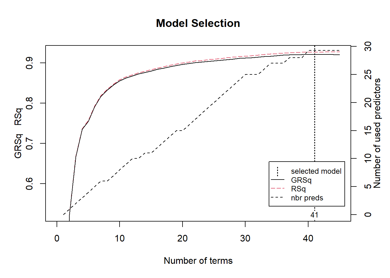
It’s also important to point out that this package has the capacity to assess potential interactions between different hinge functions.
earth(Sale_Price ~ .,
      data = ames_train,
      degree = 2) |>
  summary() |>
  (\(x) x$coefficients)() |>
  head(10)
Sale_Price
(Intercept) 3.473694e+05
h(Gr_Liv_Area-3194) 2.302940e+02
h(3194-Gr_Liv_Area) -7.005261e+01
h(Year_Built-2002) 5.242461e+03
h(2002-Year_Built) -7.360079e+02
h(Total_Bsmt_SF-2223) 1.181093e+02
h(2223-Total_Bsmt_SF) -4.901140e+01
h(Year_Built-2002)*h(Gr_Liv_Area-2398) 9.035037e+00
h(Year_Built-2002)*h(2398-Gr_Liv_Area) -3.382639e+00
h(Bsmt_Unf_SF-625)*h(3194-Gr_Liv_Area) -1.145129e-027.3.5 Tuning Process
There are two important tuning parameters associated with our MARS model:
-
degree: the maximum degree of interactions, where rarely is there any benefit in assessing greater than 3-rd degree interactions. -
nprune: Maximum number of terms (including intercept) in the pruned model, where you can start out with 10 evenly spaced values.
# create a tuning grid
hyper_grid <- expand.grid(
  degree = 1:3,
  nprune = seq(2, 100, length.out = 10) |> floor()
)

head(hyper_grid)
degree nprune
1 1 2
2 2 2
3 3 2
4 1 12
5 2 12
6 3 12Caret
# Cross-validated model
set.seed(123)  # for reproducibility
cv_mars <- train(
  x = subset(ames_train, select = -Sale_Price),
  y = ames_train$Sale_Price,
  method = "earth",
  metric = "RMSE",
  trControl = trainControl(method = "cv", number = 10),
  tuneGrid = hyper_grid
)


# View results
cv_mars$bestTune
##    nprune degree
## 16     45      2


cv_mars$results |>
  filter(nprune == cv_mars$bestTune$nprune,
         degree == cv_mars$bestTune$degree)
#   degree nprune     RMSE  Rsquared     MAE RMSESD RsquaredSD    MAESD
# 1 2 45 23427.47 0.9156561 15767.9 1883.2 0.01365285 794.2688ggplot(cv_mars)+
theme_light()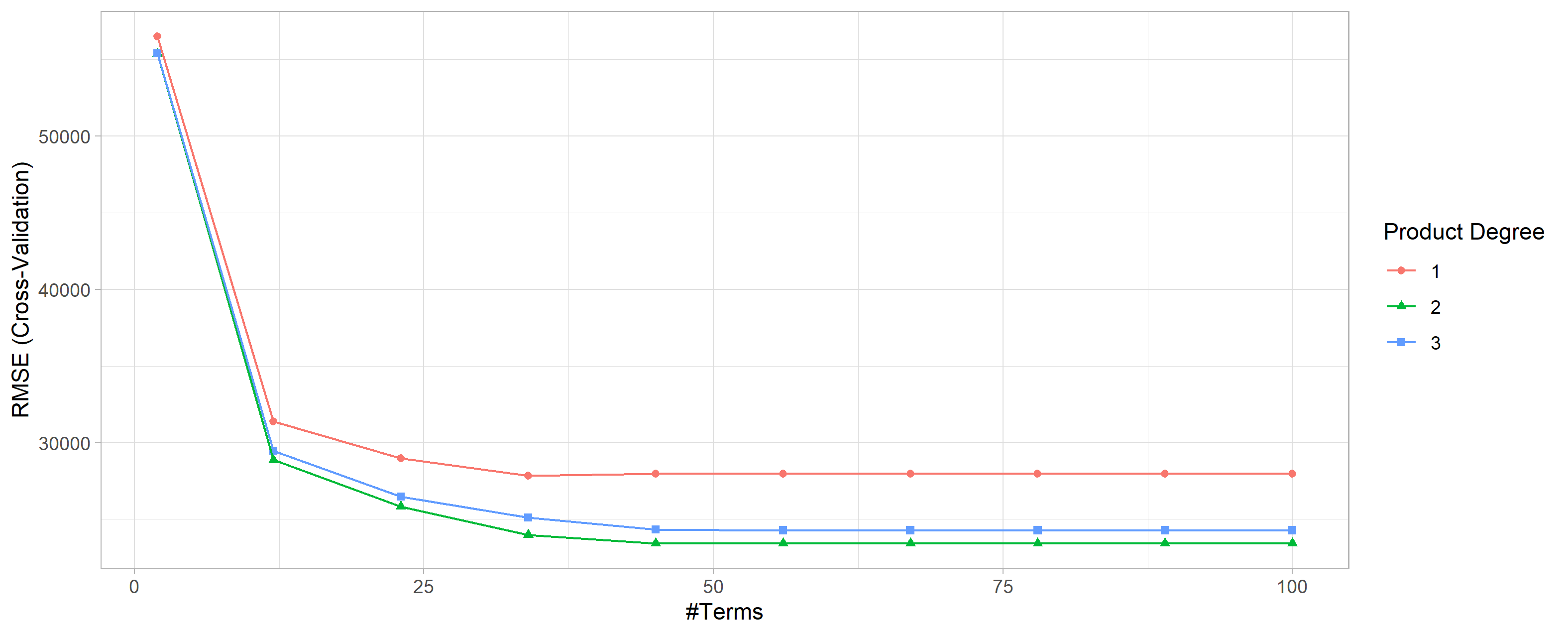
cv_mars$resample$RMSE |> summary()
#  Min. 1st Qu.  Median    Mean 3rd Qu.    Max.
# 20735   22053   23189   23427   24994   26067


cv_mars$resample
#        RMSE  Rsquared      MAE Resample
# 1  23243.22 0.9387415 15777.98   Fold04
# 2  23044.17 0.9189506 15277.56   Fold03
# 3  23499.99 0.9205506 16190.29   Fold07
# 4  23135.62 0.9226565 16106.93   Fold01
# 5  25491.41 0.8988816 16255.55   Fold05
# 6  21414.96 0.9202359 15987.68   Fold08
# 7  21722.58 0.9050642 14694.66   Fold02
# 8  26066.88 0.8938272 16635.14   Fold06
# 9  20735.28 0.9274782 14226.06   Fold10
# 10 25920.58 0.9101751 16527.20   Fold09
Tidymodels
The main benefit of using tidymodels to perform 10-CV is that you can stratify the folds, which can be very useful taking in consideration that the target variable is right-skewed.
ggplot(ames_train, aes(Sale_Price))+
  geom_histogram(fill = "blue", alpha = 0.6)+
  theme_light()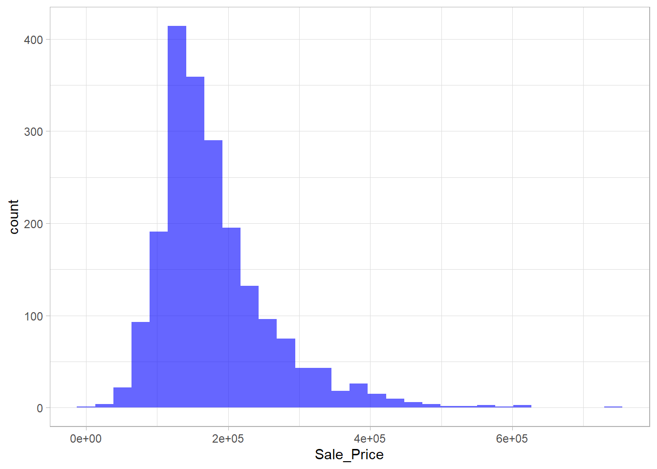
- Define the model to train
- Define the recipe to use
mars_recipe <-
  recipe(Sale_Price ~ ., data = ames_train) |>
  step_dummy(all_nominal_predictors()) |>
prep(training = ames_train) - Create a
workflowobject to join the model and recipe.
mars_wf <-
  workflows::workflow() |>
  workflows::add_recipe(mars_recipe) |>
workflows::add_model(mars_model)- Create the folds with
rsample
- Getting metrics for each resample
mars_rs_fit <-
  mars_wf |>
  tune::tune_grid(resamples = ames_folds,
                  grid = hyper_grid,
metrics = yardstick::metric_set(yardstick::rmse))- Check the winner’s parameters
mars_rs_fit |>
  tune::show_best(metric = 'rmse', n = 3)

#   nprune degree .metric .estimator   mean     n std_err .config
#    <dbl>  <int> <chr>   <chr>       <dbl> <int>   <dbl> <chr>
# 1      2      1 rmse    standard   25808.    10   1378. Preprocessor1_Model01
# 2      2      2 rmse    standard   25808.    10   1378. Preprocessor1_Model02
# 3      2      3 rmse    standard   25808.    10   1378. Preprocessor1_Model03


final_mars_wf <-
  mars_rs_fit |>
  tune::select_best(metric = 'rmse') |>
  tune::finalize_workflow(x = mars_wf)

# ══ Workflow ════════════════════════════════
# Preprocessor: Recipe
# Model: mars()
#
# ── Preprocessor ────────────────────────────
# 1 Recipe Step
#
# • step_dummy()
#
# ── Model ───────────────────────────────────
# MARS Model Specification (regression)
#
# Engine-Specific Arguments:
#   nprune = 2
#   degree = 1
#
# Computational engine: earth
7.3.6 Feature interpretation
The vip package importance will measure the impact of the prediction error as a proportion of the total error features are included (Generalized cross-validation).
# variable importance plots
p1 <-
  vip(cv_mars, num_features = 40, geom = "point", value = "gcv") +
  ggtitle("GCV")

p2 <-
  vip(cv_mars, num_features = 40, geom = "point", value = "rss") +
  ggtitle("RSS")

gridExtra::grid.arrange(p1, p2, ncol = 2)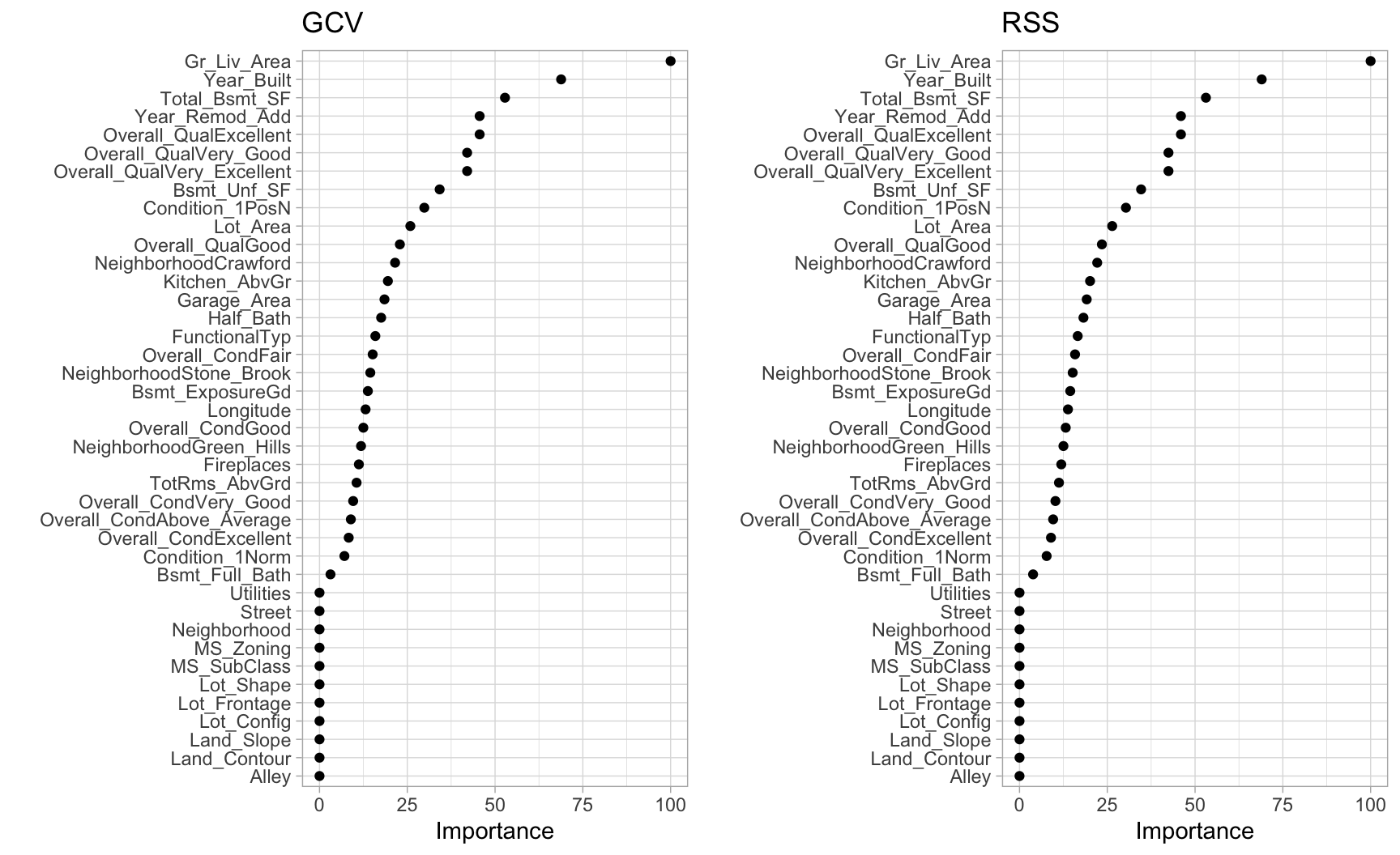
However, it does not measure the impact for particular hinge functions created for a given feature. To see the effect we need to create a plot for each predictor.
# Construct partial dependence plots
p1 <-
  partial(cv_mars, pred.var = "Gr_Liv_Area", grid.resolution = 10) |>
  autoplot()

p2 <-
  partial(cv_mars, pred.var = "Year_Built", grid.resolution = 10) |>
  autoplot()

p3 <-
  partial(cv_mars, pred.var = c("Gr_Liv_Area", "Year_Built"),
          grid.resolution = 10) %>%
  plotPartial(levelplot = FALSE, zlab = "yhat", drape = TRUE, colorkey = TRUE,
              screen = list(z = -20, x = -60))

# Display plots side by side
gridExtra::grid.arrange(p1, p2, p3, ncol = 3)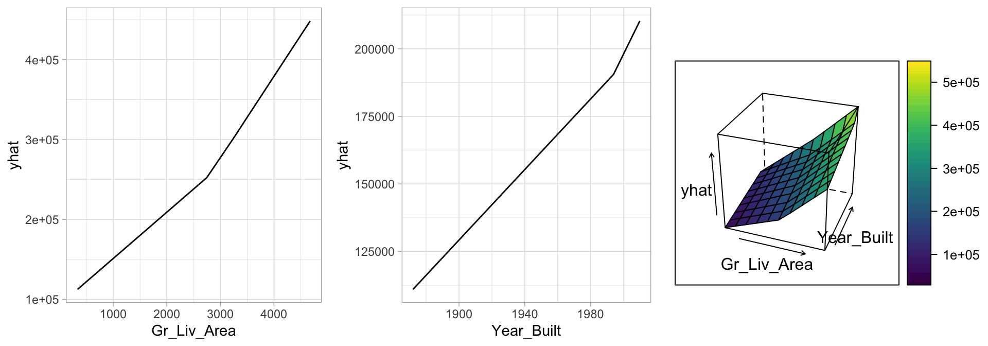
7.3.7 Final thoughts
Pros:
- Naturally handles mixed types of predictors (quantitative and qualitative)
- Requires minimal feature engineering
- Performs automated feature selection
- Highly **correlated predictors* do not impede predictive accuracy
- Finds the important nonlinear interactions present in the data
Cons:
- Slower to train
- Correlated predictors can make model interpretation difficult
7.4 K-nearest neighbors (KNN)
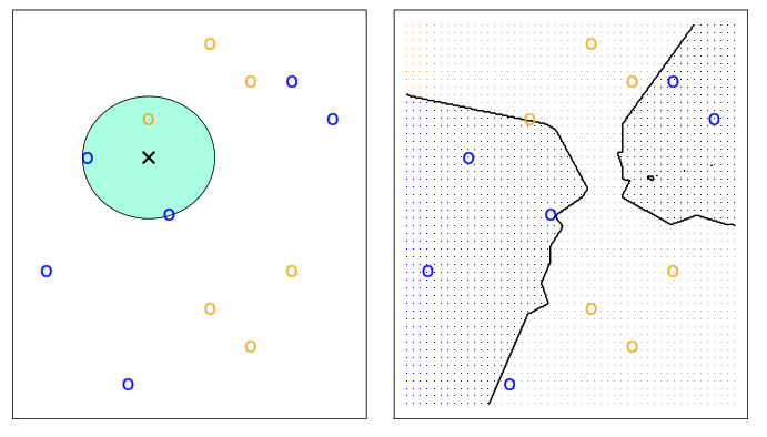
It uses the principle of nearest neighbors to classify unlabeled examples by using the Euclidean Distance to calculate distance between the point we want to predict and \(k\) closest neighbors on the training data.
\[ d\left( a,b\right) = \sqrt {\sum _{i=1}^{p} \left( a_{i}-b_{i}\right)^2 } \]
KNN unlike parametric models does not tell us which predictors are important, making it hard to make inferences using this model.
This method performs worst than a parametric as we starting adding noise predictors. In fact, we will get in the situation where for a given observation has no nearby neighbors, known as curse of dimensionality and leading to a very poor prediction of \(f(x_{0})\).
7.4.1 Classifier
The next function estimates the conditional probability for class \(j\) as the fraction of points in \(N_{0}\) whose response values equal \(j\).
\[ \text{Pr}(Y = j|X = x_{0}) = \frac{1}{K} \displaystyle\sum_{i \in N_{0}} I(y_{i} = j) \]
- Where
- \(j\) response value to test
- \(x_{0}\) is the test observation
- \(K\) the number of points in the training data that are closest to \(x_{0}\) and reduce the model flexibility
- \(N_{0}\) points in the training data that are closest to \(x_{0}\)
Then KNN classifies the test observation \(x_{0}\) to the class with the largest probability.
7.4.2 Regression
KNN regression estimates \(f(x_{0})\) using the average of all the training responses in \(N_{0}\).
\[ \hat{f}(x_{0}) = \frac{1}{K} \displaystyle\sum_{i \in N_{0}} y_{i} \]
- Where
- \(x_{0}\) is the test observation
- \(K\) the number of points in the training data that are closest to \(x_{0}\) and reduce the model flexibility
- \(N_{0}\) points in the training data that are closest to \(x_{0}\)
7.4.3 Pre-processing
To use this method we need to make sure that all our variables are numeric. If one our variables is a factor we need to perform a dummy transformation of that variable with the recipes::step_dummy function.
On the other hand, as this model uses distances to make predicts it’s important to check that each feature of the input data is measured with the same range of values with the recipes::step_range function which normalize from 0 to 1 as happens with the dummy function.
\[ x' = \frac{x - \min(x)}{\max(x) - \min(x)} \]
Another normalization alternative is centering the predictors in \(\overline{x} = 0\) with \(S = 0\) with the function recipes::step_normalize or the function scale() which apply the z-score normalization.
\[ x' = \frac{x - \mu}{\sigma} \]
7.4.4 Coding example
To perform K-Nearest Neighbors we just need to create the model specification by using kknn engine.
library(tidymodels)
library(ISLR2)

Smarket_train <-
  Smarket %>%
  filter(Year != 2005)

Smarket_test <-
  Smarket %>%
  filter(Year == 2005)

knn_spec <- nearest_neighbor(neighbors = 3) %>%
  set_mode("classification") %>%
  set_engine("kknn")

SmarketKnnPredictions <-
  knn_spec %>%
  fit(Direction ~ Lag1 + Lag2, data = Smarket_train) |>
  augment(new_data = Smarket_test)

conf_mat(SmarketKnnPredictions, truth = Direction, estimate = .pred_class)
Truth
Prediction Down Up
Down 43 58
Up 68 83accuracy(SmarketKnnPredictions, truth = Direction, estimate = .pred_class) # A tibble: 1 × 3
.metric .estimator .estimate
<chr> <chr> <dbl>
1 accuracy binary 0.57.5 Tree-Based Methods
These methods involve stratifying the predictor space into a number of simple regions and then use mean or the mode response value for the training observations in the region to which it belongs.
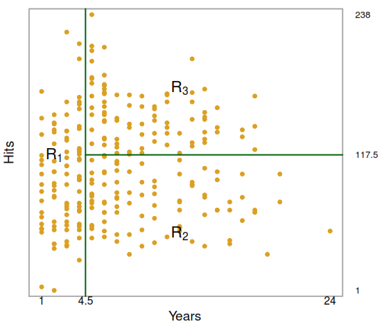
As these results can be summarized in a tree, these types of approaches are known as decision tree methods, we have some important parts:
- Terminal nodes (leaves) are represented by \(R_1\), \(R_2\) and \(R_3\).
- Internal nodes refers to the points along the tree where the predictor space is split.
- Branches refer to the segments of the trees that connect the nodes.
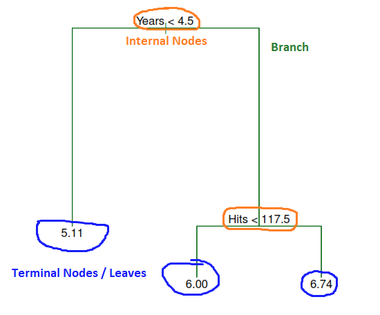
It’s important to take in consideration that the order in which is presented each predictors also explain the level of importance of each variable. For example, the number of Years has a higher effect over the player’s salary than the number of Hits.
7.5.1 Simple trees
Advantages and disadvantages
| Advantages | Disadvantages |
|---|---|
| Simpler to explain than linear regression thanks to its graphical representation | Small change in the data can cause a large change in the final estimated tree |
| It doesn’t need much preprocessing as: - It handles qualitative predictors. - It doesn’t require feature scaling or normalization. - It can handle missing values and outliers |
They aren’t so very good predicting results as: - It prones to overfitting. - It presents low accuracy. |
| It can be used for feature selection by defining the importance of a feature based on how early it appears in the tree and how often it is used for splitting | They can be biased towards the majority class in imbalanced datasets |
Regression
To create a decision tree we need to find the regions \(R_1, \dots, R_j\) that minimize the RSS where \(\hat{y}_{R_j}\) represent the mean response for the training observations within the jth box:
\[ RSS = \sum_{j=1}^J \sum_{i \in R_j} (y_i - \hat{y}_{R_j})^2 \]
To define the regions we use the recursive binary splitting, which consist the predictor \(X_j\) and the cutpoint \(s\) leads to the greatest possible reduction in RSS. Next, we repeat the process, looking for the best predictor and best cutpoint in order to split the data further so as to minimize the RSS within each of the resulting regions. The process continues until a stopping criterion is reached (no region contains more than five observations).
This method is:
Top-down: It begins at the top of the tree (where all observations belong to a single region) and then successively splits the predictor space.
Greedy: At each step of the tree-building process, the best split is made at that particular step, rather than looking ahead and picking a split that will lead to a better tree in some future step.
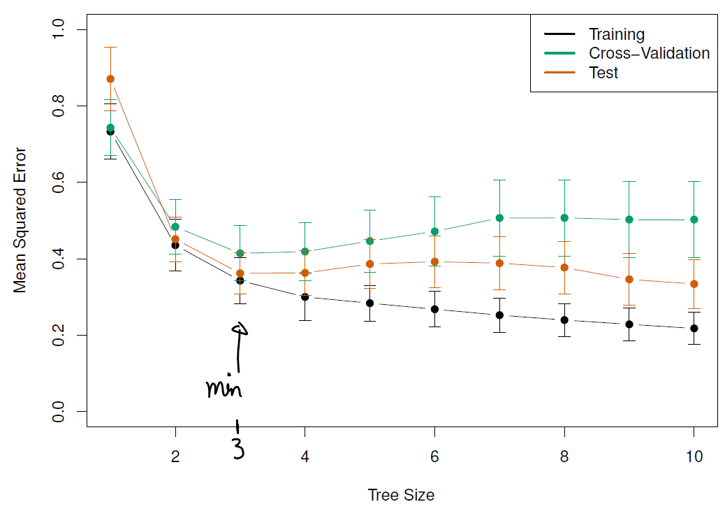
As result, we could end with a very complex tree that overfits the data. To solve this, we need prune the original tree until getting a subtree that leads to the lowest test error rate by using the cost complexity pruning approach which creates differente trees based on \(\alpha\).
\[ \sum_{m=1}^{|T|} \sum_{i: x_i \in R_m} (y_i - \hat{y}_{R_m}) ^2 + \alpha|T| \]
Where:
- \(\alpha\): Tunning parameter \([0,\infty]\) selected using k-cross validation
- \(|T|\): Number of terminal nodes of the tree \(T\).
- \(R_m\): The subset of predictor space corresponding to the \(m\)th terminal node
- \(\hat{y}_{R_m}\): Predicted response associated with \(R_m\)
Classification
For a classification tree, we predict that each observation belongs to the most commonly occurring class of training observations in the region to which it belongs.
As we can not use RSS as a criterion for making the binary splits, the classification error rate could the fraction of the training observations in that region that do not belong to the most common class (\(1 - \max_k(\hat{p}_{mk})\)), but it turns out that classification error is not sufficiently sensitive for tree-growing and we use the next metrics as they are more sensitive to node purity (proportion of the main class on each terminal node):
| Name | Formula |
|---|---|
| Gini index | \(G = \sum_{k = 1}^K 1 - \hat{p}_{mk} (1 -\hat{p}_{mk})\) |
| Entropy | \(D = -\sum_{k = 1}^K 1 - \hat{p}_{mk} \log \hat{p}_{mk}\) |
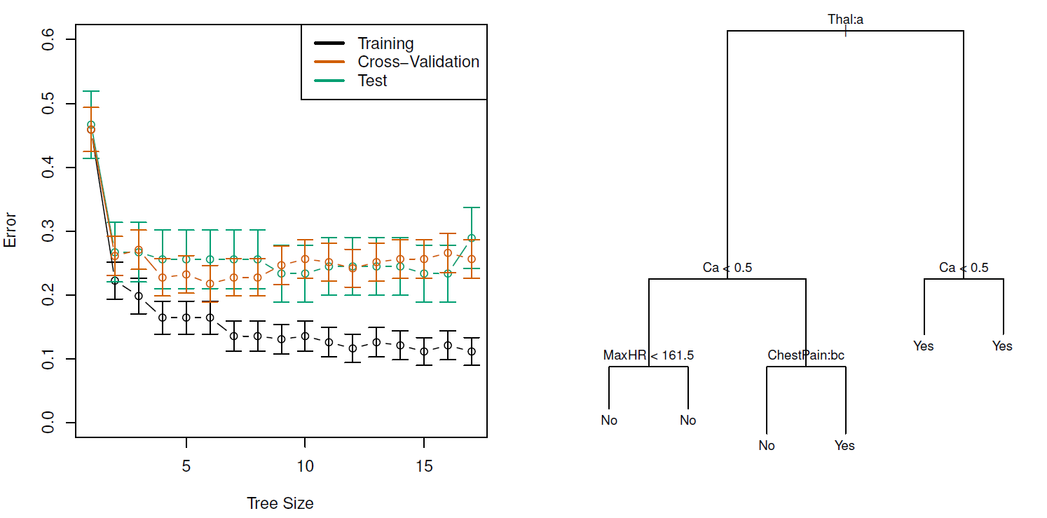
Coding example
https://app.datacamp.com/learn/tutorials/decision-trees-R
# For data maninulation
library(data.table)

# For modeling and visualization
library(tidymodels)

#
Boston <- as.data.table(MASS::Boston)

pillar::glimpse(Boston)
Rows: 506
Columns: 14
$ crim <dbl> 0.00632, 0.02731, 0.02729, 0.03237, 0.06905, 0.02985, 0.08829,…
$ zn <dbl> 18.0, 0.0, 0.0, 0.0, 0.0, 0.0, 12.5, 12.5, 12.5, 12.5, 12.5, 1…
$ indus <dbl> 2.31, 7.07, 7.07, 2.18, 2.18, 2.18, 7.87, 7.87, 7.87, 7.87, 7.…
$ chas <int> 0, 0, 0, 0, 0, 0, 0, 0, 0, 0, 0, 0, 0, 0, 0, 0, 0, 0, 0, 0, 0,…
$ nox <dbl> 0.538, 0.469, 0.469, 0.458, 0.458, 0.458, 0.524, 0.524, 0.524,…
$ rm <dbl> 6.575, 6.421, 7.185, 6.998, 7.147, 6.430, 6.012, 6.172, 5.631,…
$ age <dbl> 65.2, 78.9, 61.1, 45.8, 54.2, 58.7, 66.6, 96.1, 100.0, 85.9, 9…
$ dis <dbl> 4.0900, 4.9671, 4.9671, 6.0622, 6.0622, 6.0622, 5.5605, 5.9505…
$ rad <int> 1, 2, 2, 3, 3, 3, 5, 5, 5, 5, 5, 5, 5, 4, 4, 4, 4, 4, 4, 4, 4,…
$ tax <dbl> 296, 242, 242, 222, 222, 222, 311, 311, 311, 311, 311, 311, 31…
$ ptratio <dbl> 15.3, 17.8, 17.8, 18.7, 18.7, 18.7, 15.2, 15.2, 15.2, 15.2, 15…
$ black <dbl> 396.90, 396.90, 392.83, 394.63, 396.90, 394.12, 395.60, 396.90…
$ lstat <dbl> 4.98, 9.14, 4.03, 2.94, 5.33, 5.21, 12.43, 19.15, 29.93, 17.10…
$ medv <dbl> 24.0, 21.6, 34.7, 33.4, 36.2, 28.7, 22.9, 27.1, 16.5, 18.9, 15…7.5.2 Bagging (bootstrap aggregation)
As we said before, simple trees has a high variance problem \(Var(\hat{f}(x_{0}))\) and bagging can help to mitigate this problem.
We know from the Central Limit Theorem a natural way to reduce the variance and increase the test set accuracy is taking many training sets from the population, build a separate prediction model using each training set, and average the resulting prediction, as for a given a set of \(n\) independent observations \(Z_1, \dots, Z_n\), each with variance \(\sigma^2\), the variance of the mean \(\overline{Z}\) of the observations is given by \(\sigma^2/n\).
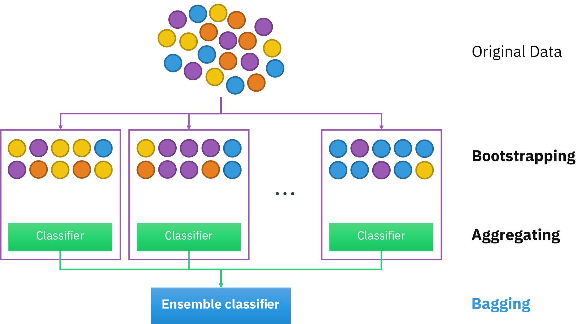
As we generally do not have access to multiple training sets we use bootstrap to take repeated samples from the one training data set, train \(B\) not pruned regression trees and average the resulting predictions or select the most commonly occurring class among the \(B\) predictions in classification settings.
\[ \hat{f}_{bag}(x) = \frac{1}{B}\sum_{b=1}^B\hat{f}^{*b}(x) \]
The number of trees is not a critical as \(B\) will not lead to overfitting. Using \(B = 100\) is sufficient to achieve good performance in this example.
Out-of-bag error estimation
To estimate the test error as an approximation of the Leave-one-out cross validation when \(B\) sufficiently large, we can take advantage of the \(1/3\) of observation that were out-of-bag (OOB) on each re-sample and predict the response for the \(i\)th observation using each of the trees in which that observation was OOB.
This will yield around \(B/3\) predictions for each of the \(n\) observation that we can average or take a majority vote to calculate the test error.
Variable importance measures
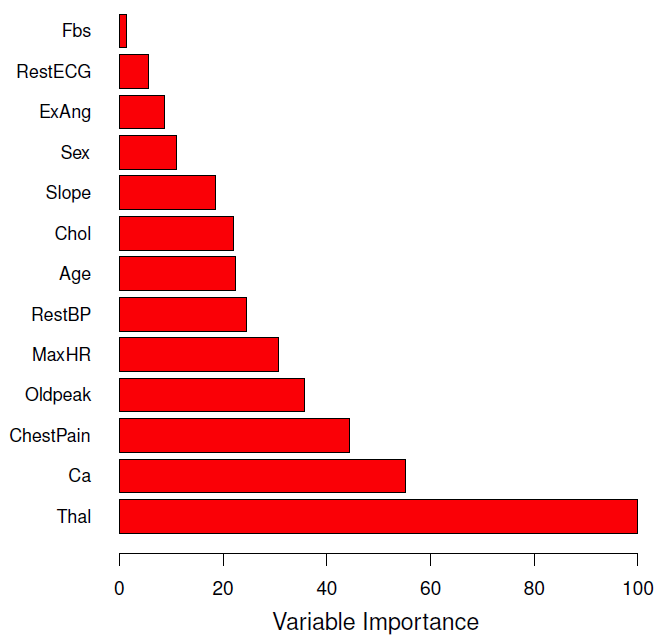
After using this method, we can’t represent the statistical learning procedure using a single tree, instead we can use the RSS (or the Gini index) to record the total amount that the RSS is decreased due to splits over a given predictor, averaged(or added) over all \(B\) trees where a large value indicates an important predictor.
7.5.3 Random Forests
Predictions from the bagged trees, has a big problem, there are highly correlated and averaging many highly correlated quantities does not lead to as large of a reduction in variance as averaging many uncorrelated quantities (independent).
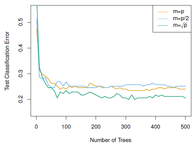
To solve this problem Random Forests provide an improvement over bagged trees by decorrelates the trees. As in bagging, we build many trees based on bootstrapped training samples. But when building these decision trees random forest sample \(m \approx \sqrt{p}\) predictors to create \(B\) *independent trees, making the average of the resulting trees less variable and hence more reliable.
Parameters to tune
Random forests have the least variability in their prediction accuracy when tuning, as the default values tend to produce good results.
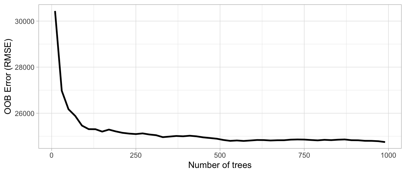
- Number of trees (\(B\)): A good rule of thumb is to start with 10 times the number of features as the error estimate converges after some trees and computation time increases linearly with the number of trees.
-
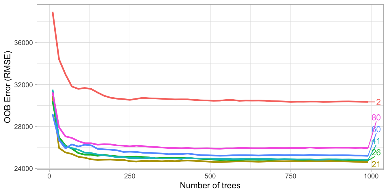
Number of predictors (\(m_{try}\)): In
ranger, \(m_{try} = \text{floor} \left( \frac{p}{3} \right)\) in regression problems and \(m_{try} = \text{floor} \left( \sqrt{p} \right)\) in classifications problems, but we can explore in the range \([2,p]\).
- With few relevant predictors (e.g., noisy data) a higher number tends to perform better because it makes it more likely to select those features with the strongest signal.
- With many relevant predictors a lower number might perform better.
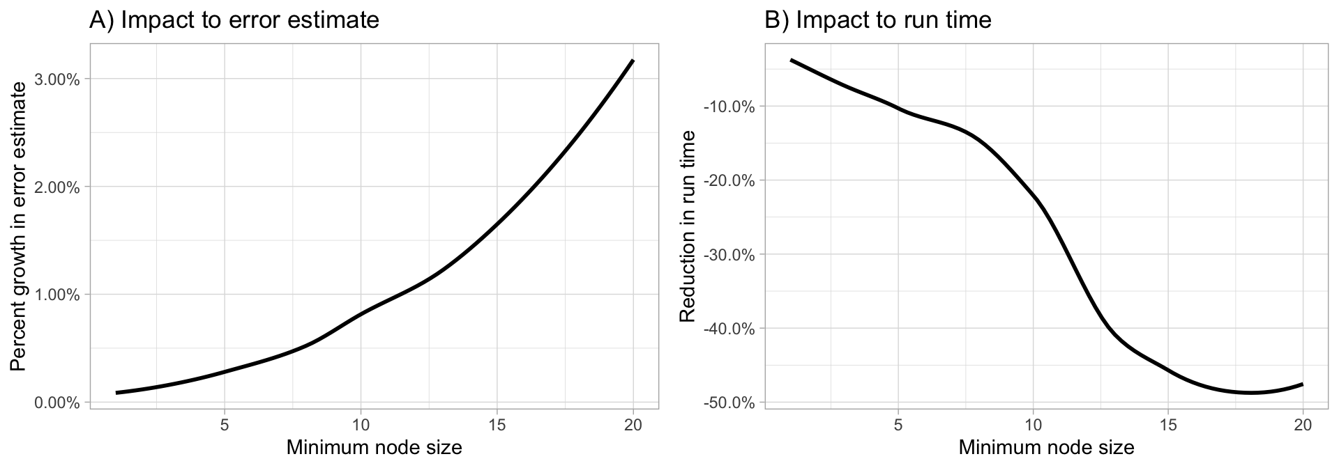
- Tree complexity (node size): The default values of \(1\) for classification and \(5\) for regression as these values tend to produce good results, but:
- If your data has many noisy predictors and a high number of trees, then performance may improve by increasing node size (i.e., decreasing tree depth and complexity).
- If computation time is a concern then you can often decrease run time substantially by increasing the node size.
Start with three values between 1–10 and adjust depending on impact to accuracy and run time.
7.5.4 Boosting
As well as bagging, boosting is a general approach that can be be applied to many statistical learning methods for regression or classification. Both methods create many models in order to create a single prediction \(\hat{f}^1, \dots, \hat{f}^B\).
To create boosting trees, in general, we need to create then sequentially by using information from prior models and fit a new model with a modified version of the original data set. To be more specific we need to flow the following steps:
Set \(\hat{f}(x) = 0\) and \(r_i=y_i\) for all \(i\) in the training set.
For \(b = 1, 2, \dots, B\), repeat the next process:
- Fit a tree \(\hat{f}^b\) with d splits (d + 1 terminal nodes) to the training data (\(X,r\)). In this step is very import to see that we are fitting the new model based on the residuals.
- Update \(\hat{f}\) by adding in a shrunken version of the new tree:
\[ \hat{f}(x) \leftarrow \hat{f}(x) + \lambda \hat{f}^b(x) \]
- Update the residuals
\[ r_i \leftarrow r_i - \lambda \hat{f}^b(x_i) \]
- Calculate the output of the boosting model by:
\[ \hat{f}(x) = \sum_{b=1}^B \lambda \hat{f}^b(x) \]
As result, our model learn slowly by adding new decision trees into the fitted function in order to update the residuals on each step. As we are going to use many models, each individual model can be small by using a low \(d\) parameter. In general, statistical learning approaches that learn slowly tend to perform well.
Parameters to tune
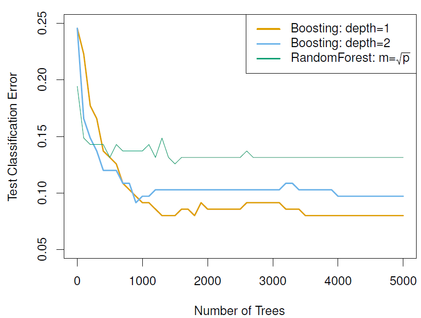
Number of trees (\(B\)): Unlike bagging and random forests, boosting can overfit if B is too large.
shrinkage (\(\lambda\)): Controls the rate at which boosting learns, it should be a positive value its values are \(0.01\) or \(0.001\). Very small \(\lambda\) can require using a very large value of B in order to achieve good performance.
Number of splits or interaction depth (\(d\)): It controls the complexity of the boosted ensemble. When \(d=1\) is known as a stump tree as each term involves only a single variable. Some times, stump tree works well and are eraser to interpret, but as \(d\) increases the number of variables used by each model increases, with \(d\) as limit.
7.5.5 Bayesian additive regression trees (BART)
This method constructs trees in a random manner as in bagging and random forests, and each tree tries to capture signal not yet accounted for by the current model, as in boosting.
To understand the method works we need to define some important notation:
- \(K\): Number of regression trees. For example \(K\) could be \(100\)
- \(B\): Number of iterations. For example \(B\) could be \(1000\)
- \(\hat{f}_k^b(x)\): The prediction at \(x\) for the \(k\)th regression tree used in the \(b\)th iteration
- \(\hat{f}^b(x) = \sum_{k=1}^K \hat{f}_k^b(x)\): Summed of the \(K\) at the end of each iteration.
To apply this method we need to follow the below steps:
- In the first iteration all trees are initialized to have a single root node,the mean of the response values divided by the total number of trees, in other to predict the mean of \(y\) in the first iteration \(\hat{f}^1(x)\).
\[ \hat{f}_k^1(x) = \frac{1}{nK} \sum_{i=1}^n y_i \]
- Compute the predictions of the first iteration.
\[ \hat{f}^1(x) = \sum_{k=1}^K \hat{f}_k^1(x) = \frac{1}{n} \sum_{i=1}^n y_i \]
- For each of the following iterations \(b = 2, \dots, B\).
-
Update each tree \(k = 1, 2, \dots, K\) by:
- Computing a partial residual for each tree with all trees but the \(k\)th tree.
\[ r_i = y_i - \sum_{k'<k} \hat{f}_{k'}^b(x_i) - \sum_{k'>k} \hat{f}_{k'}^{b-1}(x_i) \]
- Based on the partial residual BART randomly choosing a perturbation to the tree from the previous iteration \(\hat{f}_k^{b-1}\) from a set of possible perturbations (adding branches, prunning branches or changing the prediction of terminal nodes) favoring ones that improve the fit to the partial residual. This guards against overfitting since it limits how “hard” we fit the data in each iteration.
- Compute \(\hat{f}^b(x) = \sum_{k=1}^K \hat{f}_k^b(x)\)
- Compute the mean or a percentile after \(L\) burn-in iterations that don’t provide good results. For example \(L\) could be \(200\)
\[ \hat{f}(x) = \frac{1}{B-L} \sum_{b=L+1}^B \hat{f}(x) \]
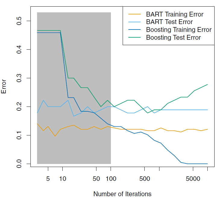
This models works really well even without a tuning process and the random process modifications protects the metho to overfit as we increase the number of iterations, as we can see in the next chart.
7.6 Support Vector Machine
7.6.1 Maximal Margin Classifier (Hard Margin Classifier)
In a p-dimensional space, a hyperplane is a flat affine subspace of hyperplane dimension \(p − 1\).
\[ f(X)= \beta_0 + \beta_1 X_1 + \beta_2 X_2 + \dots + \beta_p X_p = 0 \]
But if a point \(X = (X_1, X_3, \dots, X_p)^T\) doesn’t satisfy that equation that equation the point would lies to one or other side the equation: - Over the hyperplane if \(\beta_0 + \beta_1 X_1 + \beta_2 X_2 + \dots + \beta_p X_p > 0\) - Under the hyperplane if \(\beta_0 + \beta_1 X_1 + \beta_2 X_2 + \dots + \beta_p X_p < 0\)
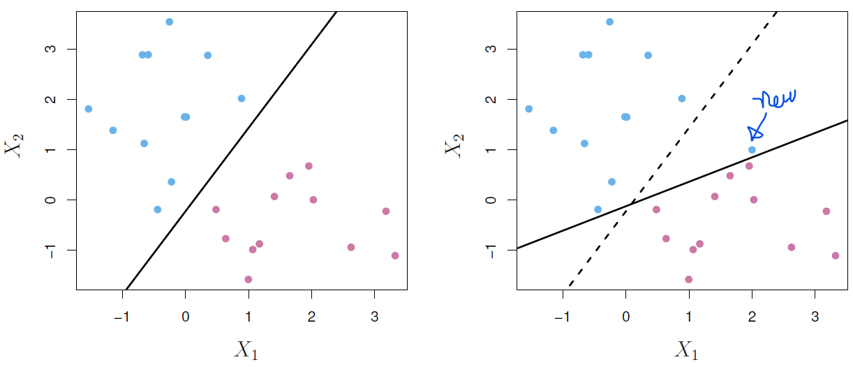
But as we can see below there are several possible hyperplane that could do the job.
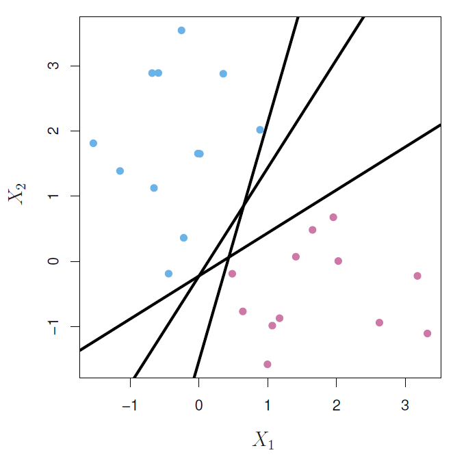
To solve this problem, we need to find the maximal margin hyperplane by computing the perpendicular distance from each training observation to a given separating hyperplane to select the farthest hyperplane from the training observations.
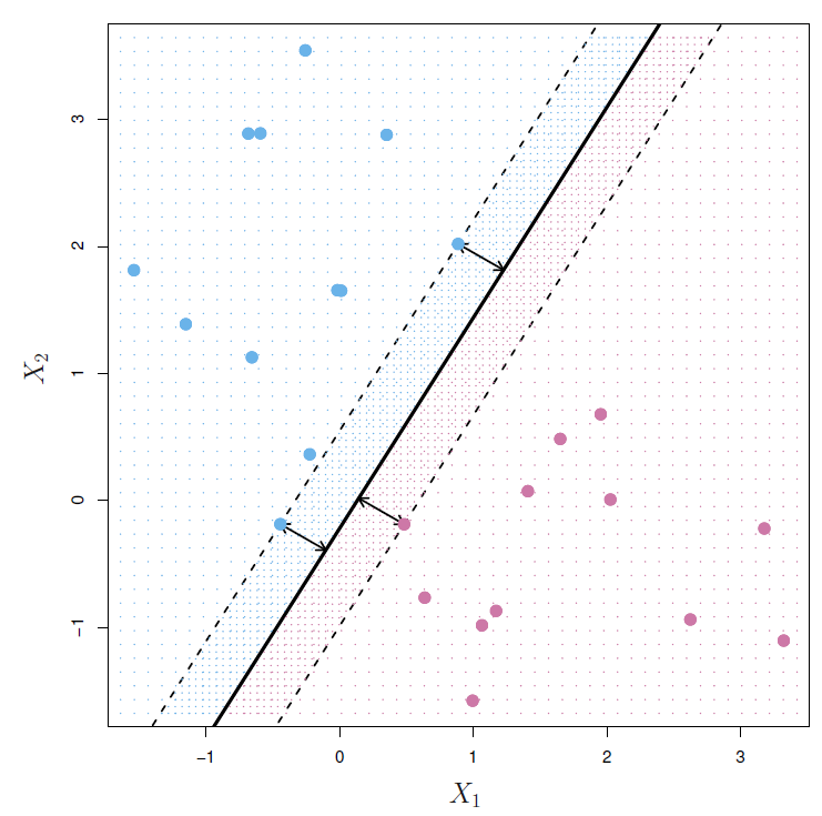
In the last example the two blue points and the purple point that lie on the dashed lines are the support vectors as they “support” the maximal margin hyperplane.
The maximal margin hyperplane is the solution to the next optimization problem where the associated class labels \(y_1, \dots, y_n \in \{-1, 1\}\):
\[ \begin{split} \underset{\beta_0, \beta_1, \dots, \beta_p}{\text{maximize}} & \; M \\ \text{subject to } & \begin{cases} \sum_{j=1}^p \beta_{j}^2 = 1 , \\ y_i(\beta_0 + \beta_1 x_{i1} + \beta_2 x_{i2} + \dots + \beta_p x_{ip}) \geq M , \; i = 1, \dots, n \end{cases} \end{split} \]
As consecuence, the ubicated in the expected side of the hyperplane will satisfafy the next condition.
\[ Y_i \times f(X) > 0 \]
This method has two disadvantages:
- Sometimes there isn’t any possible separating hyperplane.
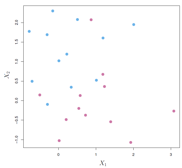
- Classifying correctly all of the training can lead to sensitivity to individual observations, returning as a result a overfitted model.
7.6.2 Support Vector Classifiers (soft margin classifier)
To solve this problem we need to allow that:
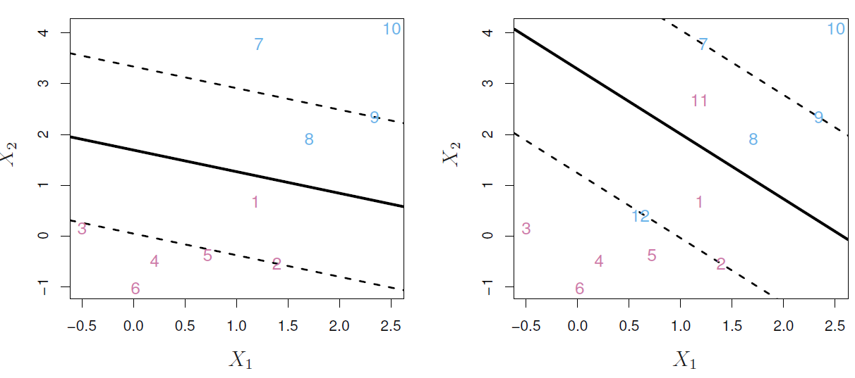
- Some observations will be on the incorrect side of the margin like observations 1 and 8.
- Some observations will be on the incorrect side of the hyperplane like observations 11 and 12.
To get that result, we need to solve the next problem:
\[ \begin{split} \underset{\beta_0, \beta_1, \dots, \beta_p, M}{\text{maximize}} & \; M \\ \text{subject to } & \begin{cases} \sum_{j=1}^p \beta_{j}^2 = 1 , \\ y_i(\beta_0 + \beta_1 x_{i1} + \beta_2 x_{i2} + \dots + \beta_p x_{ip}) \geq M (1 - \epsilon_i), \; i = 1, \dots, n \\ \epsilon_i \geq 0, \\ \sum_{i=1}^n \epsilon_i \leq C \end{cases} \end{split} \]
- Where:
- \(M\) is the width of the margin.
-
\(\epsilon_1, \dots, \epsilon_n\) are slack variables that allow individual observations to be on the wrong side of the margin or the hyperplane.
- If \(\epsilon_i = 0\) then the ith observation is on the correct side of the margin.
- If \(\epsilon_i > 0\) then the ith observation is on the wrong side of the margin.
- If \(\epsilon_i > 1\) then the ith observation is on the wrong side of the hyperplane.
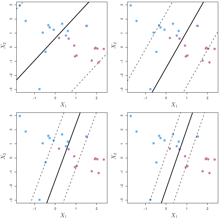
- \(C\) is a nonnegative tuning parameter that represents the budget for the total amount that the margin can be violated by the n observations. For \(C > 0\) no more than \(C\) observations can be on the wrong side of the hyperplane.
It’s important to point that only observations that either lie on the margin or violate the margin will affect the hyperplane.
7.6.3 Non-linear boundaries
To extend the Support Vector Classifier to non-lineal settings we need to use functions that quantifies the similarity of two observations, known as kernels \(K(x_i, x_{i'})\) and implement it to the hyperplane function for the support vectors \(\mathcal{S}\).
\[
f(x) = \beta_0 + \sum_{i \in \mathcal{S}} K(x_i, x_{i'})
\] And depending on the shape that we want to use there are some types of kernels to use and we need to tune the related hyperparameters. Each of the next kernels is linked to a function in tidymodelsand in the documentation of each function we will see the parameters to tune for each case
Polynomial (svm_poly)
As the degree \(d\) increases the fit becomes more non-linear.
\[ K(x_i, x_{i'}) = \alpha_i (1 + \sum_{j=1}^p x_{ij} x_{i'j})^d \]
Radial (svm_rbf)
As \(\gamma\) increases the fit becomes more non-linear.
\[ K(x_i, x_{i'}) = \exp(-\gamma \sum_{j=1}^p(x_{ij}-x_{i'j})^2) \]
Hyperbolic tangent
\[ K(x_i, x_{i'}) = \tanh(k_1||x_i-x_{i'}|| + k_2) \]
There isn’t any function to use this kernel but we can change the default kernel in the set_engine function
svm_tanh <-
  svm_linear() |>
  set_mode("classification") |>
  set_engine("kernlab",
             kernel = "tanhdot")
7.6.4 Extending SVMs to the K-class case
To extend this method we have 2 alternatives:
One-Versus-One Classification (OVO): It constructs \(\left( \begin{array}{c} K \\ 2 \end{array} \right)\), tallys the number of times that the test observation is assigned to each of the \(K\). The final classification is performed by assigning the test observation to the class to which it was most frequently assigned.
One-Versus-All Classification (OVA): We fit \(K\) SVMs, each time comparing one of the \(K\) classes to the remaining \(K − 1\) classes. Let \(\beta = \beta_{0k}, \beta_{1k}, \dots, \beta_{pk}\) denote the parameters that result from fitting an SVM comparing the \(k\)th class (coded as \(+1\)) to the others (coded as \(−1\)). We assign the observation to the class for which the lineal combination of coefficients and the test observation \(\beta x^*\) is largest.
The kernlab package support many classes by default so we don’t need to worry about this problem problem.
7.6.5 Coding Example
- Load libraries
library(tidymodels)
library(ISLR)
library(kernlab)
theme_set(theme_light())

set.seed(1)
sim_data <- tibble(
  x1 = rnorm(40),
  x2 = rnorm(40),
  y  = factor(rep(c(-1, 1), 20))
) %>%
  mutate(x1 = ifelse(y == 1, x1 + 1.5, x1),
         x2 = ifelse(y == 1, x2 + 1.5, x2))

ggplot(sim_data, aes(x1, x2, color = y)) +
  geom_point()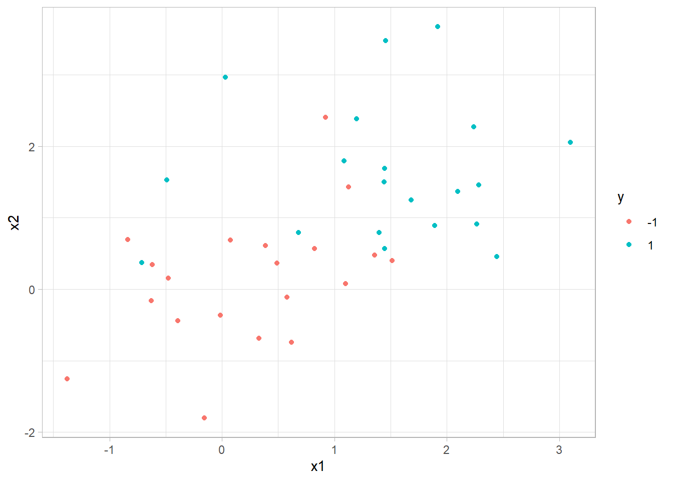
- Define model specification
svm_linear_spec <- svm_poly(degree = 1) %>%
  set_mode("classification") %>%
  # We don't need scaling for now
set_engine("kernlab", scaled = FALSE)- Fitting the model and checking results
