2 Feature Engineering
2.1 Handling Missing Values
2.1.1 Introduction
If you are working with real data, it’s normal to find missing values, so it’s very important to understand how to manage them correctly. In R, the default for many functions is to remove missing values to create plots or train machine learning models, but that can be very dangerous as we are adding bias to our analysis that could compromise our final conclusions.
But removing values could be a good option if we meet the following statements:
Only 5% of your dataset’s rows present missing values.
All the values have the same probability to be missing. That’s when we say that they are missing completely at random (MCAR).
Otherwise, the best way to handle missing values is to impute values based on general patterns found in the data. If we cannot find patterns in the current data, we will need to find more data until finding a valid pattern to impute the values.
2.1.2 Imputation practical example
Let’s assume that all the predictors for a machine learning model are stored in the datasets::airquality data frame, which has some missing values, so we need to explore and decide what to do in this case.
To perform all the tasks needed to solve the missing values problems in our dataset, we will load the following packages:
Confirming if values are MCAR
Based on the next test, we can reject the null hypothesis and conclude that the missing values aren’t completely at random, so we will need to impute the missing values.
mcar_test(airquality)# A tibble: 1 × 4
statistic df p.value missing.patterns
<dbl> <dbl> <dbl> <int>
1 35.1 14 0.00142 4Explore missing values patterns
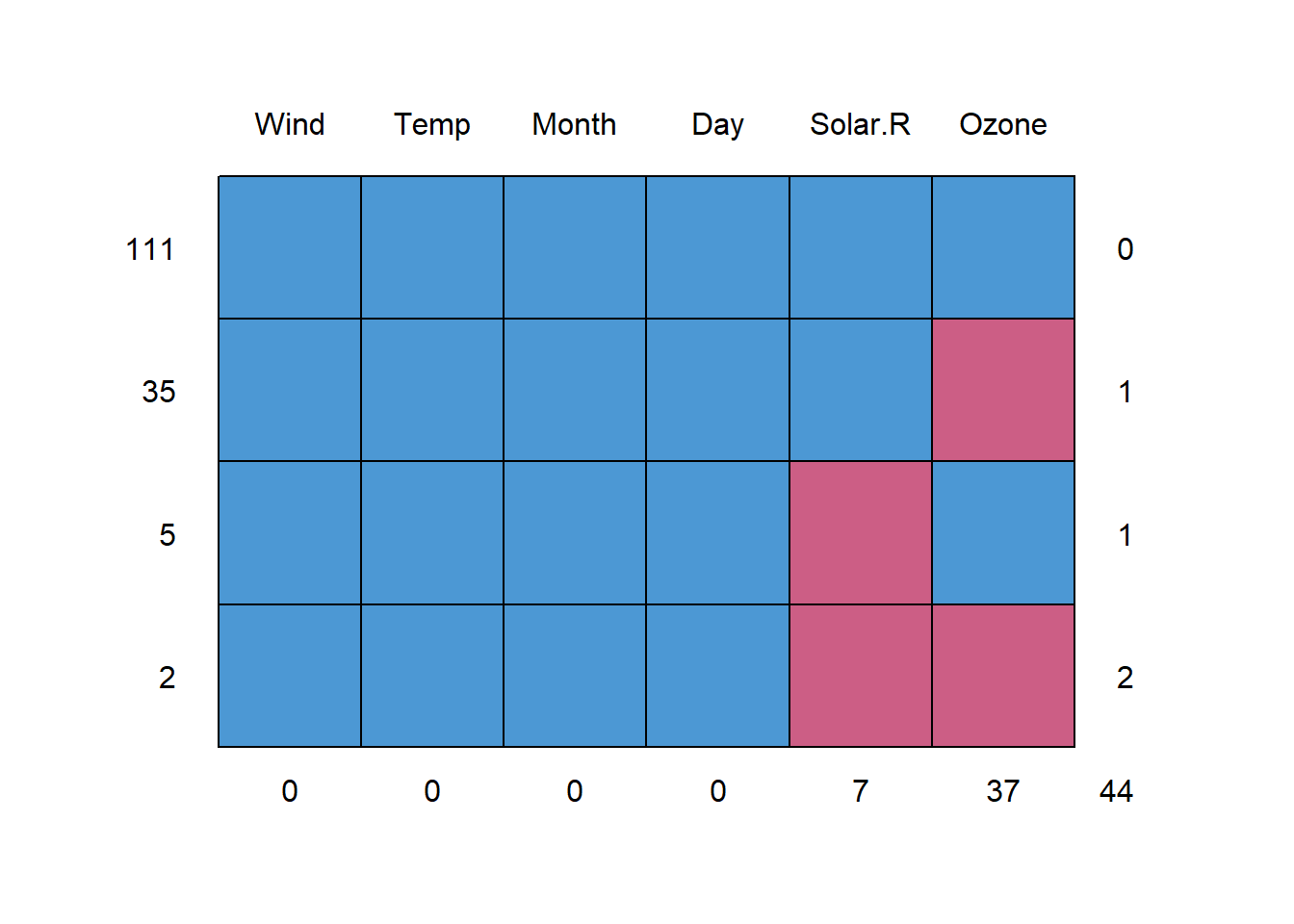
Once we know that we need to impute values, it’s important to know that the column with more missing values is the Ozone with 37 values to impute, which we can divide between the ones that can use the rest of the features (35 rows) and the ones that can use all the columns except the Solar.R as they are missing (2 rows).
airquality |>
  md.pattern() |>
  invisible()
Imputing Ozone values
Exploring missing values
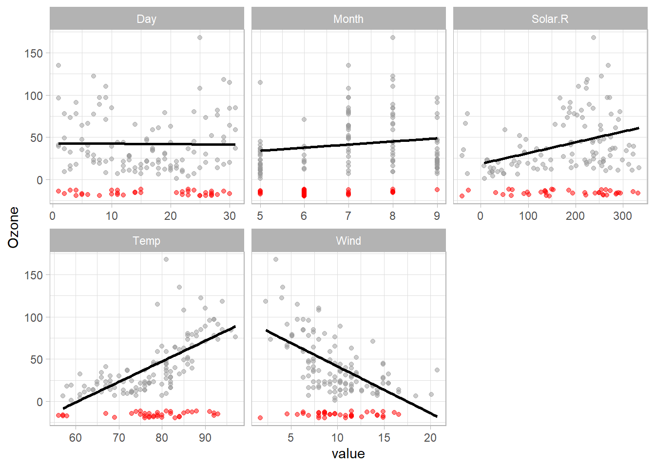
In the next plot we can see how the missing Ozone values are spread across a wide range of values, so we wouldn’t be able to find big differences between the means of columns with or without missing Ozone values.
As we are plotting all variables against the target variable, it’s easy to see that the Temp, Wind and Solar.R present a not linear relation with Ozone and we cannot see a clear pattern for Day and Month.
airquality |>
  pivot_longer(cols = -Ozone) |>
  ggplot(aes(value, Ozone))+
  geom_miss_point(aes(color = is.na(Ozone)),
                  alpha = 0.5,
                  show.legend = FALSE)+
  geom_smooth(method = "lm",
              se = FALSE,
              color = "black")+
  scale_color_manual(values = c("TRUE" = "red",
                                "FALSE" = "gray60"))+
  facet_wrap(~name, scales = "free_x")+
  theme_light()
Based on this result, we know it’s necessary to train a model able to catch the non-linear patterns and omit the Day and Month as they don’t show any relation with Ozone.
Training the model to impute
As we need to create 2 very similar models (one using the Solar.R column and other without it) it’s better to create a function.
fit_tuned_regression_model <- function(df,
                                       model_to_tune,
                                       model_grid,
                                       formula,
                                       step_fun,
                                       metric = rsq,
                                       seed = 1234){

  # Defining empty model workflow
  y_wf <-
    recipe(formula, data = df) |>
    step_fun() |>
    workflow(model_to_tune)

  # Defining re-samples based on seed
  set.seed(seed)
  y_resamples <- mc_cv(df, times = 30)
  set.seed(NULL)

  # Fitting re-sample for each grid level
  y_tuned <- tune_grid(
    y_wf,
    resamples = y_resamples,
    grid = model_grid,
    metrics = metric_set(metric)
  )

  # Selecting the best model
  y_trained_model <-
    finalize_workflow(y_wf,
                      select_best(y_tuned)) |>
    fit(df)

  # Presenting results
  results <- list("fit" = y_trained_model,
                  "best_fit" = show_best(y_tuned))

  print(results$best_fit)

  return(results)

}
Then we need to define common inputs for both models.
GlmModel <- linear_reg(
  engine = "glmnet",
  penalty = tune(),
  mixture = tune()
)

GlmGrid <- grid_regular(
  penalty(),
  mixture(),
  levels = 10
)

ozone_steps <- function(recipe){

  recipe |>
  step_poly(all_numeric_predictors(),
            degree = 2) |>
    step_interact(terms = ~(. -Ozone)^2) |>
    step_zv(all_numeric_predictors()) |>
    step_scale(all_numeric_predictors())

}
Now we can fit each model.
OzoneSolarGlmFitted <- fit_tuned_regression_model(
  df = na.omit(airquality),
  model_to_tune = GlmModel,
  model_grid = GlmGrid,
  formula = as.formula("Ozone ~ Solar.R + Temp + Wind"),
  step_fun = ozone_steps,
  seed = 5050
)
# A tibble: 5 × 8
penalty mixture .metric .estimator mean n std_err .config
<dbl> <dbl> <chr> <chr> <dbl> <int> <dbl> <chr>
1 1 1 rsq standard 0.721 30 0.0159 Preprocessor1_Mo…
2 1 0.889 rsq standard 0.721 30 0.0157 Preprocessor1_Mo…
3 1 0.778 rsq standard 0.720 30 0.0156 Preprocessor1_Mo…
4 0.0000000001 0 rsq standard 0.718 30 0.0165 Preprocessor1_Mo…
5 0.00000000129 0 rsq standard 0.718 30 0.0165 Preprocessor1_Mo…OzoneNotSolarGlmFitted <- airquality |>
select(-Solar.R) |>
na.omit() |>
fit_tuned_regression_model(model_to_tune = GlmModel,
model_grid = GlmGrid,
formula = as.formula("Ozone ~ Temp + Wind"),
step_fun = ozone_steps,
seed = 4518)# A tibble: 5 × 8
penalty mixture .metric .estimator mean n std_err .config
<dbl> <dbl> <chr> <chr> <dbl> <int> <dbl> <chr>
1 0.0000000001 0 rsq standard 0.654 30 0.0120 Preprocessor1_Mo…
2 0.00000000129 0 rsq standard 0.654 30 0.0120 Preprocessor1_Mo…
3 0.0000000167 0 rsq standard 0.654 30 0.0120 Preprocessor1_Mo…
4 0.000000215 0 rsq standard 0.654 30 0.0120 Preprocessor1_Mo…
5 0.00000278 0 rsq standard 0.654 30 0.0120 Preprocessor1_Mo…Impute missing values
Once we have both models, we can impute the Ozone values, but let’s also create a function to perform this task as we will need to repeat the process very time we need to predict a new value.
impute_ozone <- function(df,
                         solar_model,
                         no_solar_model){

  mutate(df,
         Ozone_NA = is.na(Ozone),
         Ozone = case_when(
           !is.na(Ozone) ~ Ozone,
           !is.na(Solar.R)~
             predict(solar_model, new_data = df)$.pred,
           TRUE ~
             predict(no_solar_model, new_data = df)$.pred)
  )
}


AirOzoneImputed <- impute_ozone(
  airquality,
  solar_model = OzoneSolarGlmFitted$fit,
  no_solar_model = OzoneNotSolarGlmFitted$fit
)
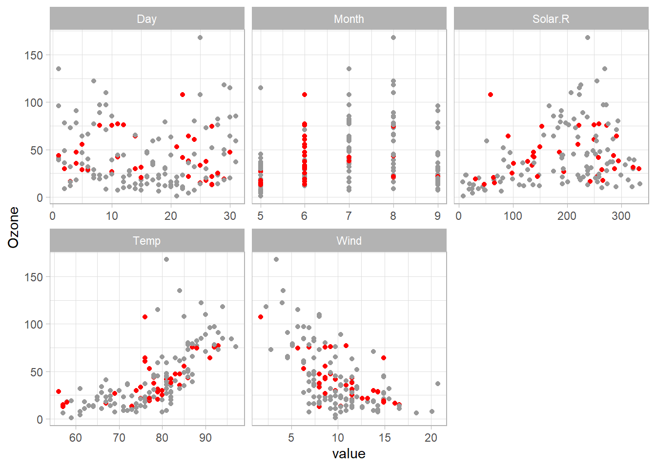
By plotting the imputed Ozone values can see that the values follow the patterns present in the non-missing values.
Fixing Solar.R values
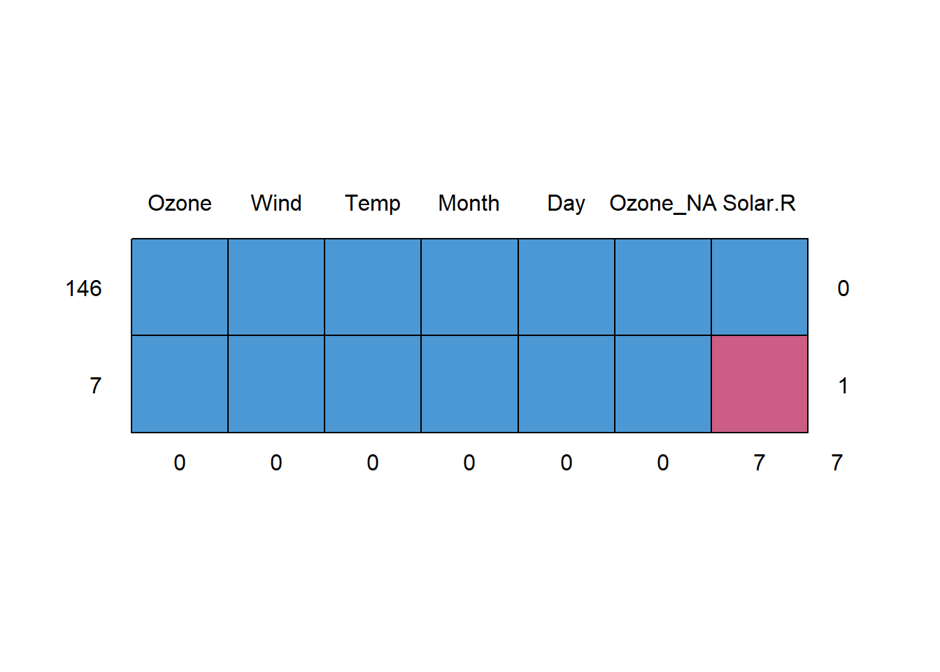
Once we don’t have any missing value in the Ozone column we can explore the remaining 7 missing values in the Solar.R column.
AirOzoneImputed |>
  md.pattern() |>
  invisible()
Now the missing values represent only 5% of the rows.
And we don’t have enough data to reject the null hypothesis, and we can not affirm that the missing values are not missing completely at random.
mcar_test(AirOzoneImputed)# A tibble: 1 × 4
statistic df p.value missing.patterns
<dbl> <dbl> <dbl> <int>
1 10.3 6 0.114 2So we can remove the remaining missing values.
2.1.3 Final thoughts
I hope this blog can help to improve your ability to handle missing values without compromising your results.
Don’t forget to explore well your columns as missing values are usually encoded with 0 or 99.
