Defining Baseline

Defining the baseline from the available data is challenging because the data lack a unique identifier for direct estimation. However, we can run a simulation to estimate the baseline value together with a confidence interval.

Simulation Assumptions

The simulation is built on the following assumptions regarding taxi drivers:

They can start working:
- From any zone in Manhattan, Brooklyn, or Queens (the most active boroughs).
- In any month, on any weekday, and at any hour.
The TLC license number (taxi company) must remain constant for all trips within a workday.
Only wheelchair‑accessible vehicles can accept trips that request a wheelchair‑accessible vehicle.
Because we cannot determine whether each zone has more active taxis than passengers, we assume that there are always more passengers than taxis. Consequently, each taxi driver can accept the first requested trip they encounter.
Taxis search for trips based on waiting time and accept the first trip found within an expanding radius:
- 0–1 minute: search within a 1‑mile radius.
- 1–3 minutes: if no trip is found, expand search to a 3‑mile radius.
- 3–5 minutes: if still no trip, expand to a 5‑mile radius.
- Continue adding 2 miles every two minutes until a trip is found.
Drivers take a 30‑minute break after 4 hours of work, but only after completing the current trip.
They will accept their last trip after working 8 hours (the 30‑minute break is not counted toward the 8 hours).

Formalizing the Simulation

Based on the rules above, we define a mathematical model following the framework described by Warren B. Powell (2022) in Sequential Decision Analytics and Modeling: Modeling with Python.

Mathematical Model Definition

State variables $S_t^n$ for the $n$‑th sample
- Initial state variables $S_0^n$
  
  Variables that do not change during the simulation
  - Taxi Company ($\text{Taxi\_Company}^n$): Taken from the hvfhs_license_num variable of the sampled first trip.
  - Limit To Take Trips ($\text{Limit\_To\_Take\_Trips}^n$): The date and time after which the driver cannot accept more trips. Obtained by adding 8 hours + 30 minutes to the request_datetime of the sampled trip.
  - Time To Take Break ($\text{Time\_To\_Take\_Break}^n$): The date and time when the driver will take the 30‑minute break. Obtained by adding 4 hours to the request_datetime of the sampled trip.
  - Taxi is WAV ($\text{Taxi\_Is\_WAV}^n$): Indicates whether this taxi can accept wheelchair‑accessible trips. Taken from the wav_match_flag variable.
  Variables that change once
  - Taken Break ($\text{Taken Break}_0^n$): Starts as FALSE and changes to TRUE after the break is taken, ensuring only one break per workday.
  Initial values of time‑varying quantities
  - Initial Time ($\text{Current\_Time}_0^n$): The date and time when the initial trip ends. Computed as request_datetime + trip_time.
  - Initial Position Zone ($\text{Current\_Zone}_0^n$): The zone where the taxi is located at the start of the simulation. Because the sampled trip is treated as the driver’s first trip, we use its DOLocationID.
  - Initial Trip Time Limit ($\text{Trip\_Time\_Limit}_0^n$): The time until which the driver searches for a trip within 1 mile. Obtained as request_datetime + trip_time + 1 minute.
  - Initial Trip Distance Limit ($\text{Trip\_Dist\_Limit}_0^n$): The initial search radius of 1 mile.
  \[ \begin{aligned} S_0 = \big( &\text{Taxi\_Company}^n,\; \text{Limit\_To\_Take\_Trips}^n,\; \text{Time\_To\_Take\_Break}^n,\; \text{Taxi\_Is\_WAV}^n, \\ &\text{Taken Break}_0^n,\; \text{Current\_Time}_0^n,\; \text{Current\_Zone}_0^n,\; \text{Trip\_Time\_Limit}_0^n,\; \text{Trip\_Dist\_Limit}_0^n \big) \end{aligned} \]
- Dynamic state variables $S_t^n$
  - Current Time ($\text{Current\_Time}_t^n$): The date and time when the driver is searching for a new trip.
  - Current Position Zone ($\text{Current\_Zone}_t^n$): The zone code where the driver is currently located.
  - Taken Break ($\text{Taken Break}_t^n$): FALSE until the break is taken, then TRUE.
  - Trip Time Limit ($\text{Trip\_Time\_Limit}_t^n$): The time until which the driver searches for a trip within the current distance limit. Updated by adding 1 or 2 minutes to $\text{Current\_Time}_t^n$ depending on previous search outcomes.
  - Trip Distance Limit ($\text{Trip\_Dist\_Limit}_t^n$): The radius (in miles) within which the driver searches for the next trip. Increases as $\text{Trip\_Time\_Limit}_t^n$ moves further from $\text{Current\_Time}_t^n$.
  \[ \begin{aligned} S_t = \big( \text{Current\_Time}_t^n,\; \text{Current\_Zone}_t^n,\; \text{Taken Break}_t^n,\; \text{Trip\_Time\_Limit}_t^n,\; \text{Trip\_Dist\_Limit}_t^n \big) \end{aligned} \]
Decision variables $x_t$

The driver decides whether to accept a sampled trip based on current location and time. Hence $x_t$ is a binary variable defined by:

\[ \begin{aligned} x_t = X^\pi\left(S_t \right) \end{aligned} \]
Exogenous information $W_{t+1}$

After completing a trip, the following variables are observed:
- Trip End Time ($\text{Trip\_End\_Time}_{t+1}^n$): The date and time when the trip ends: request_datetime + trip_time.
- Trip End Zone ($\text{Trip\_End\_Zone}_{t+1}^n$): The zone where the trip ends, taken from the DOLocationID of the accepted trip.
- Trip Earning ($\text{Trip\_Earning}_{t+1}^n$): The total earnings from the trip: driver_pay + tips.
\[ \begin{aligned} W_{t+1} = \big( \text{Trip\_End\_Time}_{t+1}^n,\; \text{Trip\_End\_Zone}_{t+1}^n,\; \text{Trip\_Earning}_{t+1}^n \big) \end{aligned} \]
Transition function $S^M(S_t, x_t, W_{t+1})$

After a trip is taken, the state variables are updated as follows:

\[ \text{Current\_Time}_{t+1}^n = \text{Trip\_End\_Time}_{t+1}^n \]

\[ \text{Current\_Zone}_{t+1}^n = \text{Trip\_End\_Zone}_{t+1}^n \]

\[ \text{Taken Break}_{t+1}^n = \text{Current\_Time}_{t+1}^n > \text{Time\_To\_Take\_Break}^n \]

\[ \text{Trip\_Time\_Limit}_{t+1}^n = \text{Current\_Time}_{t+1}^n + 1 \; \text{min} \]

\[ \text{Trip\_Dist\_Limit}_{t+1}^n = \text{Current\_Zone}_{t+1}^n + 1 \; \text{mile} \]
Objective function

Because we are not optimizing at this stage, we do not define an objective function for the baseline.

Uncertainty Model

Uncertainty in earnings arises solely from the different initial settings, which are randomly sampled to produce $N$ scenarios.

Designing Policies

The baseline policy is simply to accept any trip:

\[ X^\pi\left(S_t \right) = 1 \]

Evaluating Policies

To evaluate this policy, we estimate the total hours worked and the hourly wage for each simulated driver:

Total worked time (hours) for each initial setting:

\[ \text{Hours\_Worked}^n = \text{DropoffTime}*{\max}^n - \text{RequestTime}*{\min}^n \]
Daily hourly wage for each setting:

\[ \text{Daily\_Hourly\_Wage}^n = \frac{ \sum_{t=0}^{T^n} \left( \text{Trip\_Earning}_{t+1}^n \right) }{ \text{Hours\_Worked}^n } \]
Estimated performance of the baseline policy (average over $N$ simulated days):

\[ \hat{F}^{\pi} = \frac{1}{N} \sum_{n=1}^{N} \text{Daily\_Hourly\_Wage}^n \]

Running trips simulation

Loading the functions to use.

library(here)
library(scales)
library(ggplot2)
library(data.table)
library(lubridate)
library(infer)
library(DBI)
library(duckdb)
library(glue)
library(pins)
library(qs2)

## Custom functions
devtools::load_all()

## Defining the print params to use in the report
options(datatable.print.nrows = 15, digits = 4)

# Defining the pin boards to use
BoardLocal <- board_folder(here("../NycTaxiPins/Board"))

Creating a connection with DuckDB.

con <- dbConnect(duckdb(), dbdir = here("../NycTaxiBigFiles/my-db.duckdb"))

Importing the definition of each code zone.

ZoneCodesRef <- BoardLocal |> pin_read("ZoneCodesRef")

ZoneCodesRef[, LocationID := as.integer(LocationID)]

As most of the trips take place between Manhattan, Brooklyn and Queens, let’s list all possible combinations of related locations to use it as filter later.

ZoneCodesFilter <-
  ZoneCodesRef[
    c("Manhattan", "Brooklyn", "Queens"),
    on = "Borough",
    CJ(PULocationID = LocationID, DOLocationID = LocationID)
  ]

Selecting at random the first trip of each simulation. It’s important to know that even after setting the seed 3518 the sample is not reproducible, so we need to save the on disk to keep using the same data.

# Addig ZoneCodesFilters to db
dbWriteTable(con, "ZoneCodesFilter", ZoneCodesFilter)

# Sampling 60 trips from db
SimulationStartDayQuery <- "
SELECT t1.*
FROM NycTrips t1
INNER JOIN ZoneCodesFilter t2
  ON t1.PULocationID = t2.PULocationID AND
     t1.DOLocationID = t2.DOLocationID
WHERE t1.year = 2023
USING SAMPLE reservoir(60 ROWS) REPEATABLE (3518);
"
SimulationStartDay <- dbGetQuery(con, SimulationStartDayQuery)
setDT(SimulationStartDay)

# Saving results
BoardLocal |> pin_write(SimulationStartDay, "SimulationStartDay", type = "qs2")

pillar::glimpse(SimulationStartDay)

Rows: 60
Columns: 28
$ trip_id              <dbl> 231484989, 438922689, 295887990, 362960205, 34445…
$ hvfhs_license_num    <chr> "HV0003", "HV0005", "HV0003", "HV0003", "HV0003",…
$ dispatching_base_num <chr> "B03404", "B03406", "B03404", "B03404", "B03404",…
$ originating_base_num <chr> "B03404", NA, "B03404", "B03404", "B03404", "B034…
$ request_datetime     <dttm> 2023-02-01 23:56:37, 2023-12-21 15:37:47, 2023-0…
$ on_scene_datetime    <dttm> 2023-02-01 23:59:42, NA, 2023-05-12 19:36:15, 20…
$ pickup_datetime      <dttm> 2023-02-02 00:00:50, 2023-12-21 15:43:09, 2023-0…
$ dropoff_datetime     <dttm> 2023-02-02 00:08:37, 2023-12-21 16:03:57, 2023-0…
$ PULocationID         <dbl> 130, 50, 191, 132, 74, 232, 145, 142, 181, 137, 2…
$ DOLocationID         <dbl> 121, 229, 101, 255, 116, 228, 157, 161, 112, 225,…
$ trip_miles           <dbl> 1.520, 2.257, 4.440, 15.720, 2.340, 8.180, 3.060,…
$ trip_time            <dbl> 467, 1248, 865, 3044, 1353, 1711, 1448, 455, 1934…
$ base_passenger_fare  <dbl> 9.74, 20.79, 16.74, 46.71, 14.28, 32.48, 18.82, 1…
$ tolls                <dbl> 0.00, 0.00, 0.00, 0.00, 0.00, 0.00, 0.00, 0.00, 0…
$ bcf                  <dbl> 0.29, 0.57, 0.50, 1.35, 0.39, 0.97, 0.52, 0.32, 0…
$ sales_tax            <dbl> 0.86, 1.84, 1.49, 4.37, 1.27, 2.88, 1.67, 1.03, 2…
$ congestion_surcharge <dbl> 0.00, 2.75, 0.00, 0.00, 0.00, 0.75, 0.00, 2.75, 0…
$ airport_fee          <dbl> 0.0, 0.0, 0.0, 2.5, 0.0, 0.0, 0.0, 0.0, 0.0, 0.0,…
$ tips                 <dbl> 0.00, 0.00, 0.00, 5.49, 0.00, 0.00, 0.00, 0.00, 0…
$ driver_pay           <dbl> 6.65, 14.83, 14.03, 49.77, 15.79, 26.84, 19.54, 5…
$ shared_request_flag  <chr> "N", "N", "N", "N", "N", "Y", "N", "N", "N", "N",…
$ shared_match_flag    <chr> "N", "N", "N", "N", "N", "N", "N", "N", "N", "N",…
$ access_a_ride_flag   <chr> " ", "N", " ", " ", " ", " ", " ", "N", "N", "N",…
$ wav_request_flag     <chr> "N", "N", "N", "N", "N", "N", "N", "N", "N", "N",…
$ wav_match_flag       <chr> "N", "N", "N", "N", "N", "N", "N", "N", "N", "N",…
$ month                <chr> "02", "12", "05", "08", "07", "06", "10", "08", "…
$ year                 <dbl> 2023, 2023, 2023, 2023, 2023, 2023, 2023, 2023, 2…
$ performance_per_hour <dbl> 51.26, 42.78, 58.39, 65.35, 42.01, 56.47, 48.58, …

We can also confirm that the sample satisfy the initial restrictions:

All trips are from 2023.

SimulationStartDay[, .N, year]

    year     N
   <num> <int>
1:  2023    60

The trips begin on the expected boroughs.

ZoneCodesRef[
  SimulationStartDay,
  on = c("LocationID" = "PULocationID"),
  .N,
  by = "Borough"
]

     Borough     N
      <char> <int>
1:    Queens    15
2: Manhattan    25
3:  Brooklyn    20

The trips end on the expected boroughs.

ZoneCodesRef[
  SimulationStartDay,
  on = c("LocationID" = "DOLocationID"),
  .N,
  by = "Borough"
]

     Borough     N
      <char> <int>
1:    Queens    18
2: Manhattan    20
3:  Brooklyn    22

Now we can conclude that the initial data satisfy the assumption 1.

Calculating the mean distance present from one location to other if it has fewer than 7 miles.

MeanDistanceQuery <- "
CREATE TABLE PointMeanDistance AS

-- Selecting all avaiable from trips that don't start and end at same point
WITH ListOfPoints AS (
  SELECT 
    t1.PULocationID,
    t1.DOLocationID,
    AVG(t1.trip_miles) AS trip_miles_mean
  FROM 
    NycTrips t1
  INNER JOIN
    ZoneCodesFilter t2
    ON t1.PULocationID = t2.PULocationID AND
       t1.DOLocationID = t2.DOLocationID
  WHERE
    t1.PULocationID <> t1.DOLocationID AND
    t1.year = 2023
  GROUP BY 
    t1.PULocationID, 
    t1.DOLocationID
  HAVING 
    AVG(t1.trip_miles) <= 7
),

-- Defining all available distances
ListOfPointsComplete AS (
  SELECT
    PULocationID,
    DOLocationID,
    trip_miles_mean
  FROM ListOfPoints
  UNION ALL
  SELECT
    DOLocationID AS PULocationID,
    PULocationID AS DOLocationID,
    trip_miles_mean
  FROM ListOfPoints
),
NumeredRows AS (
  SELECT
    PULocationID,
    DOLocationID,
    trip_miles_mean,
    row_number() OVER (PARTITION BY PULocationID, DOLocationID) AS n_row
  FROM ListOfPointsComplete
)

-- Selecting the first combination of distances
SELECT 
  PULocationID,
  DOLocationID,
  trip_miles_mean
FROM NumeredRows
WHERE n_row = 1
ORDER BY PULocationID, trip_miles_mean;
"

# Saving table on DB for simulation
dbExecute(con, MeanDistanceQuery)

# Saving the table as a file
PointMeanDistance <- 
  dbGetQuery(con, "SELECT * FROM PointMeanDistance") |>
  data.table::as.data.table()

BoardLocal |> pin_write(PointMeanDistance, "PointMeanDistance", type = "qs2")

Running the simulation.

SimulationHourlyWage <- simulate_trips(con, SimulationStartDay)

pin_write(
  LocalBoard,
  SimulationHourlyWage,
  "SimulationHourlyWage",
  type = "qs2"
)

Disconnecting from DB.

dbDisconnect(con, shutdown = TRUE)

Showing simulation results.

DailyHourlyWage <-
  SimulationHourlyWage[,
    .(
      `Daily Hourly Wage` = sum(sim_driver_pay + sim_tips) /
        as.double(difftime(
          max(sim_dropoff_datetime),
          min(sim_request_datetime),
          units = "hours"
        ))
    ),
    by = "simulation_id"
  ]


DailyHourlyWage |>
  ggplot() +
  geom_histogram(aes(`Daily Hourly Wage`), bins = 10) +
  scale_x_continuous(breaks = breaks_width(10)) +
  theme_light()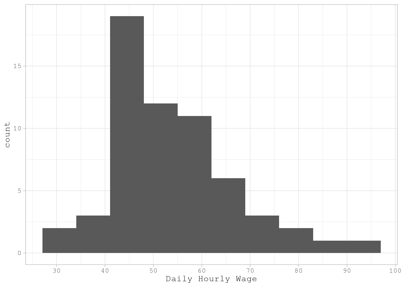

Defining a Condifence Interval

After simulating 60 days, we can use bootstrap to infer the distribution of the mean Daily Hourly Wage for any day in the year by following the next steps.

Resample with replacement a new 60 days hourly wage 3,000 times and calculate the mean of each resample.

set.seed(1586)

BootstrapHourlyWage <-
  specify(DailyHourlyWage, `Daily Hourly Wage` ~ NULL) |>
  generate(reps = 3000, type = "bootstrap") |>
  calculate(stat = "mean")

BootstrapHourlyWage

Response: Daily Hourly Wage (numeric)
# A tibble: 3,000 × 2
   replicate  stat
       <int> <dbl>
 1         1  55.1
 2         2  53.5
 3         3  53.2
 4         4  52.8
 5         5  54.2
 6         6  53.1
 7         7  54.3
 8         8  53.4
 9         9  54.3
10        10  52.6
# ℹ 2,990 more rows

Compute the 95% confident interval.

BootstrapInterval <-
  get_ci(BootstrapHourlyWage, level = 0.95, type = "percentile")

BootstrapInterval

# A tibble: 1 × 2
  lower_ci upper_ci
     <dbl>    <dbl>
1     50.5     57.1

Visualize the estimated distribution.

visualize(BootstrapHourlyWage) +
  shade_ci(endpoints = BootstrapInterval, color = "#2c77BF", fill = "#2c77BF") +
  annotate(
    geom = "text",
    y = 400,
    x = c(BootstrapInterval[1L][[1L]] - 0.4, BootstrapInterval[2L][[1L]] + 0.4),
    label = unlist(BootstrapInterval) |> comma(accuracy = 0.01)
  ) +
  labs(title = "Mean Hourly Wage Distribution", y = "Count") +
  theme_light() +
  theme(
    panel.grid.minor.y = element_blank(),
    panel.grid.major.y = element_blank(),
    plot.title = element_text(face = "bold"),
    axis.title.x = element_blank()
  )

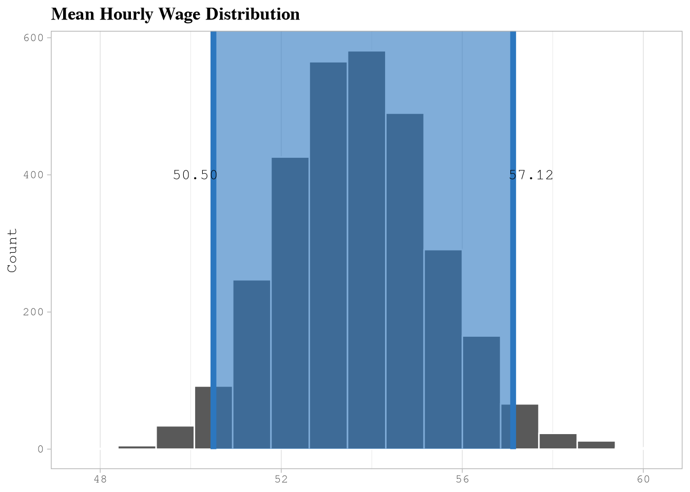
Business Case

Based on the simulation’s results we can confirm that the average earnings for a taxi driver per hour goes between 50.5 and 57.12, but that doesn’t represent the highest values observed on the simulation.

If we can check the simulation results we can confirm that a 25% of the simulated days presented earnings over the 60 dollars per hour.

GoalRate <-
  DailyHourlyWage$`Daily Hourly Wage` |>
  quantile(probs = 0.75) |>
  unname() |>
  round(2)

GoalRate

[1] 60.46

If we can apply a strategy that can move the Daily Hourly Wage to 60.46 dollars per hour, assuming the the taxi driver works 5 days every week for 8 hours, that would mean a increase of $1,593.37 every month.