Business Understanding

Project Name

Increasing NYC Taxi Drivers Earnings.

Problem Statement

Taxi drivers could increase their earnings by changing the strategy to select the trips to take, and zone and time to start working.

Project Objective

Develop a model to increase NYC taxi drivers’ hourly earnings by 20% through optimal trip selection.

Project Scope

This project will be limited to Juno, Uber, Via and Lyft taxi drivers who work in New York City in trips that take place between any zone of Manhattan, Brooklyn or Queens (the more active ones).

Stakeholders

• Taxi drivers
• Taxi companies
• Customers
• NYC Taxi and Limousine Commission

Top Process Definition

The elements of the process are defined using a SIPOC diagram.

Data to Use

In this project, we will use a subset of the data available in the TLC Trip Record Data from 2022 to 2023 for High Volume For-Hire Vehicle with the columns described below in the data dictionary.

Field Name	Description
hvfhs_license_num	The TLC license number of the HVFHS base or business. As of September 2019, the HVFHS licensees are the following: - HV0002: Juno - HV0003: Uber - HV0004: Via - HV0005: Lyft
dispatching_base_num	The TLC Base License Number of the base that dispatched the trip
originating_base_num	Base number of the base that received the original trip request
request_datetime	Date/time when passenger requested to be picked up
on_scene_datetime	Date/time when driver arrived at the pick-up location (Accessible Vehicles-only)
pickup_datetime	The date and time of the trip pick-up
dropoff_datetime	The date and time of the trip drop-off
PULocationID	TLC Taxi Zone in which the trip began
DOLocationID	TLC Taxi Zone in which the trip ended
trip_miles	Total miles for passenger trip
trip_time	Total time in seconds for passenger trip
base_passenger_fare	Base passenger fare before tolls, tips, taxes, and fees
tolls	Total amount of all tolls paid in trip
bcf	Total amount collected in trip for Black Car Fund
sales_tax	Total amount collected in trip for NYS sales tax
congestion_surcharge	Total amount collected in trip for NYS congestion surcharge
airport_fee	$2.50 for both drop off and pick up at LaGuardia, Newark, and John F. Kennedy airports
tips	Total amount of tips received from passenger
driver_pay	Total driver pay (not including tolls or tips and net of commission, surcharges, or taxes)
shared_request_flag	Did the passenger agree to a shared/pooled ride, regardless of whether they were matched? (Y/N)
shared_match_flag	Did the passenger share the vehicle with another passenger who booked separately at any point during the trip? (Y/N)
access_a_ride_flag	Was the trip administered on behalf of the Metropolitan Transportation Authority (MTA)? (Y/N)
wav_request_flag	Did the passenger request a wheelchair-accessible vehicle (WAV)? (Y/N)
wav_match_flag	Did the trip occur in a wheelchair-accessible vehicle (WAV)? (Y/N)

Based on the variables available, we can divide them into 2 categories:

Available Before Arriving at the Pick-Up Location

They will be used as the predictors to train the model and can be divided into 2 groups:

1. Fixed during the experiment as they can not be changed from trip to trip.

• hvfhs_license_num
• wav_match_flag

2. Valid for changing from trip to trip.

• request_datetime
• PULocationID
• DOLocationID
• airport_fee
• base_passenger_fare
• trip_miles
• shared_request_flag
• access_a_ride_flag
• wav_request_flag
• dispatching_base_num
• originating_base_num

Available After Ending the Trip

They can be used to create the outcome variable needed to be predicted by the model.

• dropoff_datetime
• driver_pay
• tips
• on_scene_datetime
• pickup_datetime
• congestion_surcharge
• trip_time
• tolls
• bcf
• sales_tax
• shared_match_flag

Defining Business Metric

Based on the current information, we can say that our objective is to increase the Daily Hourly Wage received by each taxi driver defined by the following formula:

\[ \text{Daily Hourly Wage} = \frac{\text{Total Earnings}}{\text{Total Hours Worked}} \]

Defining Metric’s Base Line

Defining the baseline based on this data is a challenge as the data doesn’t have any unique id to make the estimation, but we can run a simulation to estimate its value with a confident interval.

The simulation will be based on the following assumptions related to the taxi drivers:

1. They can start to work:

• From any zone of Manhattan, Brooklyn or Queens (the more active ones)
• From any month, weekday or hour.

2. The TLC license number (taxi company) needs to keep constant for all trips in workday.

3. Only wheelchair-accessible vehicles can accept trips with that request.

4. As we cannot estimate whether each zone have more active taxis than passengers we will assume that there is always more passengers than taxis and each taxi driver can accept the first requested trip.

5. The taxis will find trips based on their time waiting and will take the first trip in their valid radius:

• 0-1 Minute: Search within a 1-mile radius.
• 1-3 Minutes: Expand search to a 3-mile radius if no trip is found.
• 3-5 Minutes: Expand search to a 5-mile radius if still no trip is found.
• Keep adding 2 miles every two minutes until finding a trip.

6. They have a 30 minutes break after 4 hours working once ending the current trip.

7. They will take their last trip after working 8 hours, without taking into consideration the 30 minutes break.

Running trips simulation

1. Loading the functions to use.

library(here)
library(scales)
library(ggplot2)
library(data.table)
library(lubridate)
library(infer)
library(DBI)
library(duckdb)
library(glue)

options(datatable.print.nrows = 15)

2. Creating a connection with DuckDB.

con <- dbConnect(duckdb(), dbdir = here("my-db.duckdb"))

3. Importing the definition of each code zone.

ZoneCodesRef <- fread(
  here("raw-data/taxi_zone_lookup.csv"),
  colClasses = c("integer",
                 "character",
                 "character",
                 "character"),
  data.table = TRUE,
  key = "Borough"
)[, Address := paste(Zone,
                     Borough,
                     "New York",
                     "United States",
                     sep = ", ")
][, tidygeocoder::geocode(.SD,
                          address = Address,
                          method = 'arcgis')]

setDT(ZoneCodesRef)

dbWriteTable(con, "ZoneCodesRef", ZoneCodesRef)

BoroughColors <- c(
  'Manhattan' = '#e41a1c',
  'Queens' = '#377eb8',
  'Brooklyn'= '#4daf4a',
  'Bronx' = '#984ea3',
  'Staten Island' = '#ff7f00',
  'EWR' = '#a65628'
)

plot_map(
  ZoneCodesRef,
  lng_var = "long",
  lat_var = "lat",
  color_var = "Borough",
  color_palette = BoroughColors,
  radius = 3,
  label_var = "Zone"
)

4. As we saw before there are we need to fix some problems with the locations.

ZoneCodesRefClean <- copy(ZoneCodesRef)

# Corrected by looking the location on Google Maps
ZoneCodesRefClean[Zone == "Bloomingdale",
                  c("lat", "long") := .(40.7987912430794, 
                                        -73.96978865023877)]

ZoneCodesRefClean[Zone == "Newark Airport",
                  c("lat", "long") := .(40.689499,
                                        -74.174484)]

ZoneCodesRefClean[Zone == "Governor's Island", 
                  c("lat", 'long') := .(40.68759208028148,
                                        -74.02010657167092)]

ZoneCodesRefClean[Zone == "Ellis Island", 
                  c("lat", 'long') := .(40.69930943708351,
                                        -74.03975375195799)]

ZoneCodesRefClean[Zone == "Liberty Island", 
                  c("lat", 'long') := .(40.689975518189954,
                                        -74.04541235583368)]

# Consolidating Zone names with same locations
ZoneCodesRefClean[, Zone := data.table::fcase(
  LocationID %in% c(7L, 179L),
  "(Old) Astoria",
  
  LocationID %in% c(21L, 22L),
  "Bensonhurst (East|West)",
  
  LocationID %in% c(36L, 37L),
  "Bushwick (North|South)",
  
  LocationID %in% c(41L, 42L),
  "Central Harlem (North)",
  
  LocationID %in% c(48L, 50L),
  "Clinton (East|West)",
  
  LocationID %in% c(61L, 62L),
  "Crown Heights (North|South)",
  
  LocationID %in% c(71L, 72L),
  "East Flatbush (Farragut|Remsen Village)",
  
  LocationID %in% c(74L, 75L),
  "East Harlem (North|South)",
  
  LocationID %in% c(82L, 83L),
  "Elmhurst (Maspeth)",
  
  LocationID %in% c(87L, 88L),
  "Financial District (North|South)",
  
  LocationID %in% c(113L, 114L),
  "Greenwich Village (North|South)",
  
  LocationID %in% c(140L, 141L),
  "Lenox Hill (East|West)",
  
  LocationID %in% c(142L, 143L),
  "Lincoln Square (East|West)",
  
  LocationID %in% c(158L, 249L),
  "(Meatpacking) West Village",
  
  LocationID %in% c(177L, 178L),
  "Ocean (Hill|Parkway South)",
  
  LocationID %in% c(218L, 219L),
  "Springfield Gardens (North|South)",
  
  LocationID %in% c(227L, 228L),
  "Sunset Park (East|West)",
  
  LocationID %in% c(236L, 237L),
  "Upper East Side (North|South)",
  
  LocationID %in% c(238L, 239L),
  "Upper West Side (North|South)",
  
  LocationID %in% c(262L, 263L),
  "Yorkville (East|West)",
  
  LocationID %in% c(264L, 265L),
  "NA",
  
  rep(TRUE, times = .N), 
  Zone
)]

plot_map(
  ZoneCodesRefClean,
  lng_var = "long",
  lat_var = "lat",
  color_var = "Borough",
  color_palette = BoroughColors,
  radius = 3,
  label_var = "Zone"
)

Now we can save the results in the database.

dbWriteTable(con, "ZoneCodesRefClean", ZoneCodesRefClean)

5. Creating and saving a temporal table listing all possible combinations of locations in Manhattan, Brooklyn and Queens (they have more trips that other borough in NYC) to be used as filter.

ZoneCodesFilter <-
  ZoneCodesRefClean[c("Manhattan", "Brooklyn", "Queens"), 
                    on = "Borough",
                    CJ(PULocationID = LocationID,
                       DOLocationID = LocationID)]

dbWriteTable(con, "ZoneCodesFilter", ZoneCodesFilter)

5. Selecting at random the first trip of each simulation. It’s important to know that even after setting the seed 3518 the sample is not reproducible, so I saved the data as part of the package of this project, so you have a easy access by running proyect.nyc.taxi::SimulationStartDay, this why creating the trip_id column was so important.

SimulationStartDayQuery <- "
SELECT t1.*
FROM NycTrips t1
INNER JOIN ZoneCodesFilter t2
  ON t1.PULocationID = t2.PULocationID AND
     t1.DOLocationID = t2.DOLocationID
WHERE t1.year = 2023
USING SAMPLE reservoir(60 ROWS) REPEATABLE (3518);
"

SimulationStartDay <- dbGetQuery(con, SimulationStartDayQuery)

setDT(SimulationStartDay)

pillar::glimpse(SimulationStartDay)

#> Rows: 60
#> Columns: 28
#> $ trip_id              <dbl> 218799831, 260042034, 260089720, 295417701, 33294…
#> $ hvfhs_license_num    <chr> "HV0005", "HV0003", "HV0003", "HV0003", "HV0003",…
#> $ dispatching_base_num <chr> "B03406", "B03404", "B03404", "B03404", "B03404",…
#> $ originating_base_num <chr> NA, "B03404", "B03404", "B03404", "B03404", "B034…
#> $ request_datetime     <dttm> 2023-01-12 20:14:29, 2023-03-17 18:50:16, 2023-0…
#> $ on_scene_datetime    <dttm> NA, 2023-03-17 18:54:32, 2023-03-17 19:19:38, 20…
#> $ pickup_datetime      <dttm> 2023-01-12 20:17:48, 2023-03-17 18:55:06, 2023-0…
#> $ dropoff_datetime     <dttm> 2023-01-12 20:25:49, 2023-03-17 19:11:35, 2023-0…
#> $ PULocationID         <dbl> 50, 80, 11, 112, 135, 76, 107, 230, 79, 210, 260,…
#> $ DOLocationID         <dbl> 230, 17, 14, 37, 10, 63, 138, 246, 198, 61, 138, …
#> $ trip_miles           <dbl> 0.993, 2.250, 4.520, 2.120, 5.370, 3.260, 9.740, …
#> $ trip_time            <dbl> 481, 989, 1732, 670, 988, 1001, 1000, 894, 2900, …
#> $ base_passenger_fare  <dbl> 8.26, 16.93, 24.00, 13.38, 20.57, 16.96, 29.59, 1…
#> $ tolls                <dbl> 0.00, 0.00, 0.00, 0.00, 0.00, 0.00, 6.94, 0.00, 0…
#> $ bcf                  <dbl> 0.25, 0.51, 0.72, 0.40, 0.57, 0.47, 1.07, 0.35, 1…
#> $ sales_tax            <dbl> 0.73, 1.50, 2.13, 1.19, 1.83, 1.51, 3.46, 1.13, 3…
#> $ congestion_surcharge <dbl> 2.75, 0.00, 0.00, 0.00, 0.00, 0.00, 2.75, 2.75, 2…
#> $ airport_fee          <dbl> 0.00, 0.00, 0.00, 0.00, 0.00, 0.00, 2.50, 0.00, 0…
#> $ tips                 <dbl> 0.00, 0.00, 0.00, 0.00, 3.44, 0.00, 0.00, 0.00, 1…
#> $ driver_pay           <dbl> 5.47, 13.32, 22.22, 9.09, 16.41, 13.69, 22.25, 10…
#> $ shared_request_flag  <chr> "N", "N", "N", "N", "N", "N", "N", "N", "N", "N",…
#> $ shared_match_flag    <chr> "N", "N", "N", "N", "N", "N", "N", "N", "N", "N",…
#> $ access_a_ride_flag   <chr> "N", " ", " ", " ", " ", " ", " ", " ", " ", "N",…
#> $ wav_request_flag     <chr> "N", "N", "N", "N", "N", "N", "N", "N", "N", "N",…
#> $ wav_match_flag       <chr> "N", "N", "N", "N", "N", "N", "N", "N", "N", "N",…
#> $ month                <chr> "01", "03", "03", "05", "07", "08", "09", "10", "…
#> $ year                 <dbl> 2023, 2023, 2023, 2023, 2023, 2023, 2023, 2023, 2…
#> $ performance_per_hour <dbl> 28.95882, 37.49179, 43.00645, 31.16571, 65.74057,…

We can also confirm that the sample satisfy the initial restrictions:

• All trips are from 2023.

SimulationStartDay[, .N, year]
#>     year     N
#>    <num> <int>
#> 1:  2023    60

• The trips begin on the expected boroughs.

ZoneCodesRefClean[SimulationStartDay, 
                  on = c("LocationID" = "PULocationID"),
                  .N,
                  by = "Borough"]
#>      Borough     N
#>       <char> <int>
#> 1: Manhattan    25
#> 2:  Brooklyn    22
#> 3:    Queens    13

• The trips end on the expected boroughs.

ZoneCodesRefClean[SimulationStartDay, 
                  on = c("LocationID" = "DOLocationID"),
                  .N,
                  by = "Borough"]
#>      Borough     N
#>       <char> <int>
#> 1: Manhattan    24
#> 2:  Brooklyn    17
#> 3:    Queens    19

Now we can conclude that the initial data satisfy the assumption 1.

6. Calculating the mean distance present from one location to other if it has fewer than 10 miles.

MeanDistanceQuery <- "
CREATE TABLE PointMeanDistance AS

-- Selecting all avaiable from trips that don't start and end at same point
WITH ListOfPoints AS (
  SELECT 
    t1.PULocationID,
    t1.DOLocationID,
    AVG(t1.trip_miles) AS trip_miles_mean
  FROM 
    NycTrips t1
  INNER JOIN
    ZoneCodesFilter t2
    ON t1.PULocationID = t2.PULocationID AND
       t1.DOLocationID = t2.DOLocationID
  WHERE
    t1.PULocationID <> t1.DOLocationID AND
    t1.year = 2023
  GROUP BY 
    t1.PULocationID, 
    t1.DOLocationID
  HAVING 
    AVG(t1.trip_miles) <= 7
),

-- Defining all available distances
ListOfPointsComplete AS (
  SELECT
    PULocationID,
    DOLocationID,
    trip_miles_mean
  FROM ListOfPoints
  UNION ALL
  SELECT
    DOLocationID AS PULocationID,
    PULocationID AS DOLocationID,
    trip_miles_mean
  FROM ListOfPoints
),
NumeredRows AS (
  SELECT
    PULocationID,
    DOLocationID,
    trip_miles_mean,
    row_number() OVER (PARTITION BY PULocationID, DOLocationID) AS n_row
  FROM ListOfPointsComplete
)

-- Selecting the first combination of distances
SELECT 
  PULocationID,
  DOLocationID,
  trip_miles_mean
FROM NumeredRows
WHERE n_row = 1
ORDER BY PULocationID, trip_miles_mean;
"

dbExecute(con, MeanDistanceQuery)

dbListTables(con)

7. Running the simulation.

SimulationHourlyWage <- simulate_trips(con, SimulationStartDay)

DailyHourlyWage <-
  SimulationHourlyWage[, .(`Daily Hourly Wage` = 
                             sum(sim_driver_pay + sim_tips) /
                             as.double(difftime(max(sim_dropoff_datetime), 
                                                min(sim_request_datetime),
                                                units = "hours"))),
                       by = "simulation_id"]


DailyHourlyWage |>
  ggplot()+
  geom_histogram(aes(`Daily Hourly Wage`),
                 bins = 10) +
  scale_x_continuous(breaks = breaks_width(10)) +
  theme_light()

Defining a Condifence Interval

After simulating 60 days, we can use bootstrap to infer the distribution of the mean Daily Hourly Wage for any day in the year by following the next steps.

1. Resample with replacement a new 60 days hourly wage 3,000 times and calculate the mean of each resample.

set.seed(1586)

BootstrapHourlyWage <-
  specify(DailyHourlyWage,
          `Daily Hourly Wage` ~ NULL) |>
  generate(reps = 3000, type = "bootstrap") |>
  calculate(stat = "mean")

BootstrapHourlyWage
#> Response: Daily Hourly Wage (numeric)
#> # A tibble: 3,000 × 2
#>    replicate  stat
#>        <int> <dbl>
#>  1         1  44.9
#>  2         2  44.6
#>  3         3  46.9
#>  4         4  46.7
#>  5         5  45.9
#>  6         6  46.7
#>  7         7  47.0
#>  8         8  48.7
#>  9         9  46.4
#> 10        10  47.2
#> # ℹ 2,990 more rows

2. Compute the 95% confident interval.

BootstrapInterval <- 
  get_ci(BootstrapHourlyWage, 
         level = 0.95,
         type = "percentile")

BootstrapInterval
#> # A tibble: 1 × 2
#>   lower_ci upper_ci
#>      <dbl>    <dbl>
#> 1     44.3     50.7

3. Visualize the estimated distribution.

visualize(BootstrapHourlyWage)+
  shade_ci(endpoints = BootstrapInterval,
           color = "#2c77BF",
           fill = "#2c77BF")+
  annotate(geom = "text",
           y = 400,
           x = c(BootstrapInterval[1L][[1L]] - 0.4,
                 BootstrapInterval[2L][[1L]] + 0.4),
           label = unlist(BootstrapInterval) |> comma(accuracy = 0.01))+
  labs(title = "Mean Hourly Wage Distribution",
       y = "Count")+
  theme_light()+
  theme(panel.grid.minor.y = element_blank(),
        panel.grid.major.y = element_blank(),
        plot.title = element_text(face = "bold"),
        axis.title.x = element_blank())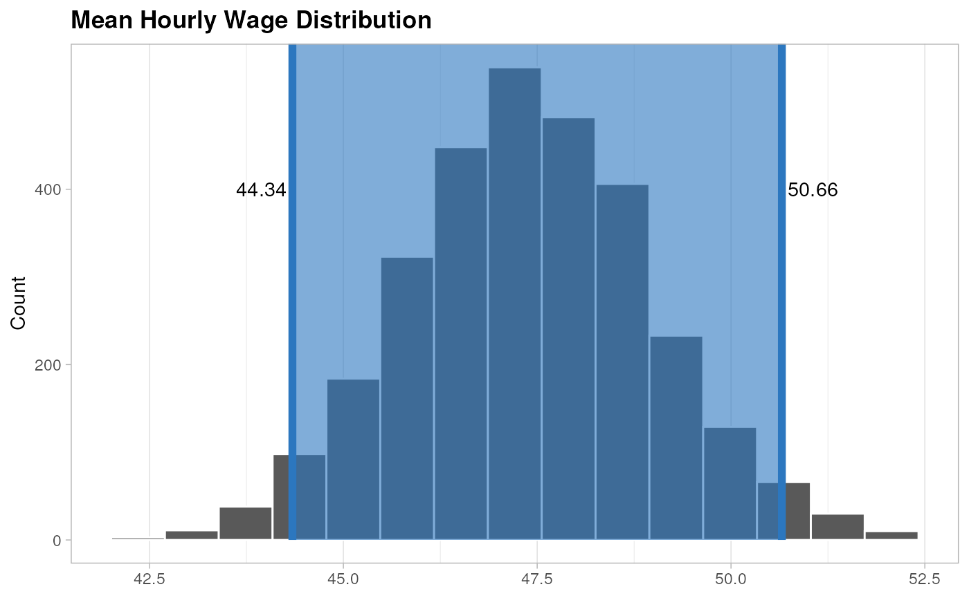

Business Case

Based on the simulation’s results we can confirm that the average earnings for a taxi driver per hour goes between 44.32 and 50.63, but that doesn’t represent the highest values observed on the simulation.

If we can check the simulation results we can confirm that a 10% of the simulated days presented earnings over the 60 dollars per hour.

DailyHourlyWage$`Daily Hourly Wage` |> 
  quantile(probs = 0.9)
#>      90% 
#> 60.95187

If we can apply a strategy that can move the Daily Hourly Wage to 60 dollars per hour ($ = 20% $) if woud be a be a great change for many taxi driver if they apply this strategy.

Ethical Considerations

While this project aims to increase taxi driver earnings, it’s important to acknowledge that optimizing for driver profits could have significant downsides:

1. Reduced service quality: Drivers focusing solely on maximizing earnings may avoid less profitable areas or times, potentially leaving some passengers underserved.

2. Discrimination risks: An earnings-focused strategy could inadvertently lead to discriminatory practices if certain demographics or neighborhoods are perceived as less profitable.

3. Increased congestion: Drivers congregating in high-profit areas could worsen traffic in already busy parts of the city.

In conclusion, this project was created to show my abilities as Data Scientist, but it is not a project that should be implemented due this considerations.

Defining Outcome to Predict

As a taxi driver only can take 2 decisions when working to increase their earnings:

1. When and where to start working.
2. Accept or reject each individual trip request.

To address the first decision, we need explore the factors that can improve the performance_per_hour of each trip.

But to address the second question, we need to create the variable best_trip_20_m which shows 1 if the current trip is the best to take in the following 20 minutes.

Deliverables

1. An HTML presentation, explaining the best places and times to start working as taxi drivers to increase your earnings.

2. A Shiny app which assists the drivers reject o accept trips to increase their earnings.